It acts by moving, through the fixed computational grid, such momentum sources as will ensure that the velocities at locations within the body have the values implied by the prescribed motion.
A recent development concerned with "domain movement" has been contributed by Dr Jeremy Wu. It is described in the Appendix: domain movement.
Pre-existing techniques
The elements of MOFOR
Implementation in PHOENICS
The next steps of development
Conclusion
Equipment for the design of which a moving-body-simulation capability is required include:
This field of endeavour, to which CFD has so far made little contribution, presents many opportunities, such as:
Phenomena of interest in this area include:
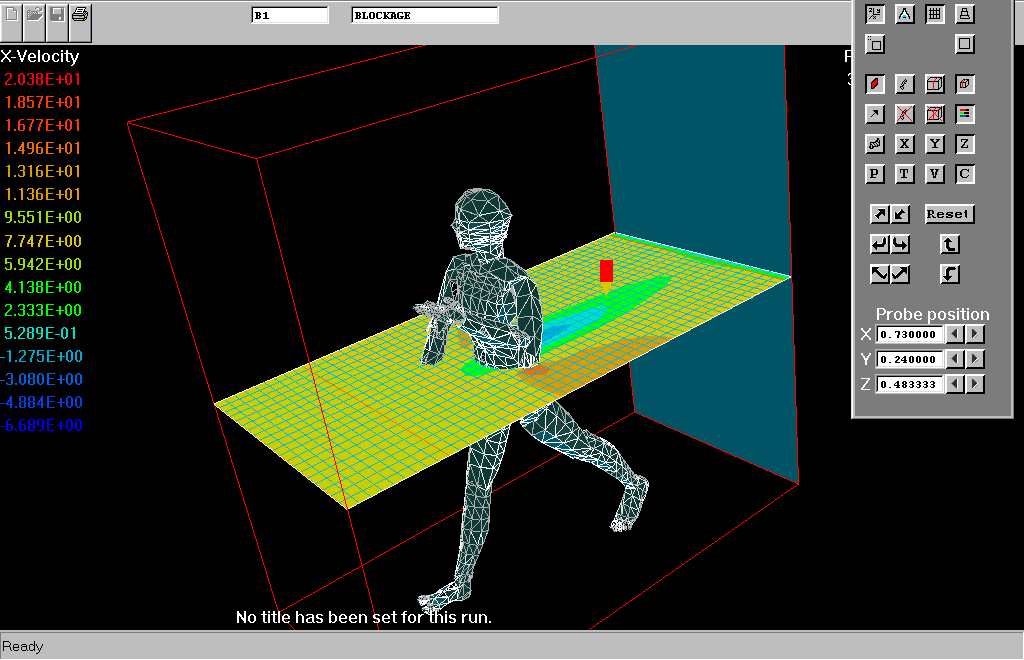
Human beings, and especially military personnel, sometimes have to move in environments which are too hot or too cold for comfort, or even survival.
It is therefore necessary to be able to provide them with protective clothing; and this is best designed with the aid of simulation software.
Such problems are complex because as well as the movement of the person's limbs relative to the surrounding atmosphere, there is motion also relative to the clothing.
Thus, air is forced along the sleeve by the flexing of an arm; and the chest expands and contracts through breathing whereas the vest does not.
Despite the difficulties, CFD is beginning to be able to make a quantitative contribution.
Common to most of the above examples are the following themes:
What is required therefore is a conceptual framework, embodied in simulation software, which can handle this wide range of phenomena.
Fortunately, when creating that framework, we did not have to start from scratch.
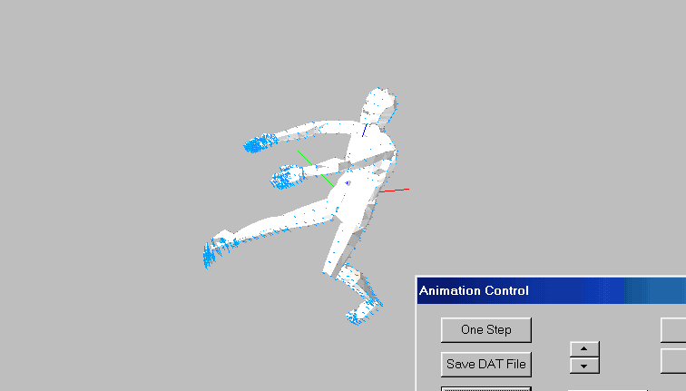
For example, the computerised film industry has encountered and solved the problem of describing, in computer-understandable terms, the motion of human and other beings;
and CHAM has made use of that means in its Bodymaker program.
Click here to see a "still" from a bodymaker "dance".
In particular, the Biovision Corporation has proposed and published
the so-called BVH ( =Biovision Hierarchical) format for describing the
motion of articulated objects, which is what human beings (in the present
context) actually are. The MOF format can be regarded as "extended BVH".
Nor of course is it the first time that PHOENICS has been used for the simulation of the fluid-dynamic effects of objects in relative motion.
The following animation sequence shows one of CHAM's first (1997) simulations of this kind.
Further,
a displacement-type compressor was among the first simulations created
by the old
ASAP procedure.
There are two main methods for describing the size and shape of solid objects, namely:
" circular cylinder with length 1m and radius 0.1m "; and
The old ASAP procedure. employed the first practice; and indeed it may well be that something of that no-longer-used procedure should be revived.
Now however the words-and-numbers method is expressed via the In-Form procedure.
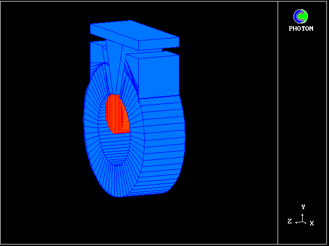
In case 768, for example, a spiral object is created by way of a simple formula.
It is also a source of heat, as the following
temperature contour shows.
The method of describing the shape and size of objects by way of facets came into use in PHOENICS with the introduction of "Virtual-reality", where it was used primarily for graphical-display purpose.
Its use continued, and indeed became deeply embedded in PHOENICS, as a means of informing the EARTH module about:
It is necessary to retain in use both methods, because:
Nevertheless it must be recognised that, where it is usable, the 'words-and-numbers' method is superior.
Thus it takes hundreds of facets to describe adequately even a simple cylinder; and each must requires three Cartesian coordinates to be supplied for each of its four vertices.
The 'words-and-numbers' method is much more compact.
Whichever method is used for describing the shape and size of an object, a single method is used for describing its position and orientation relative to the reference frame (i.e. grid) which is being used to describe the CFD cells.
Note: In BVH terminology, 'frame' is used in the cinematographic sense, as a 'shot' or 'instantaneous state'. That is not the sense used here.
This single method has the following elements, which will be described in terms of the 'bounding - box' concept:
Were all objects to move independently of one another, motion could be described by listing the values of the three translations and three rotations of the object's reference frame at successive instants of time.
However, many objects are connected together so that the movement of one enforces some movement of the another. Such objects are here called articulated.
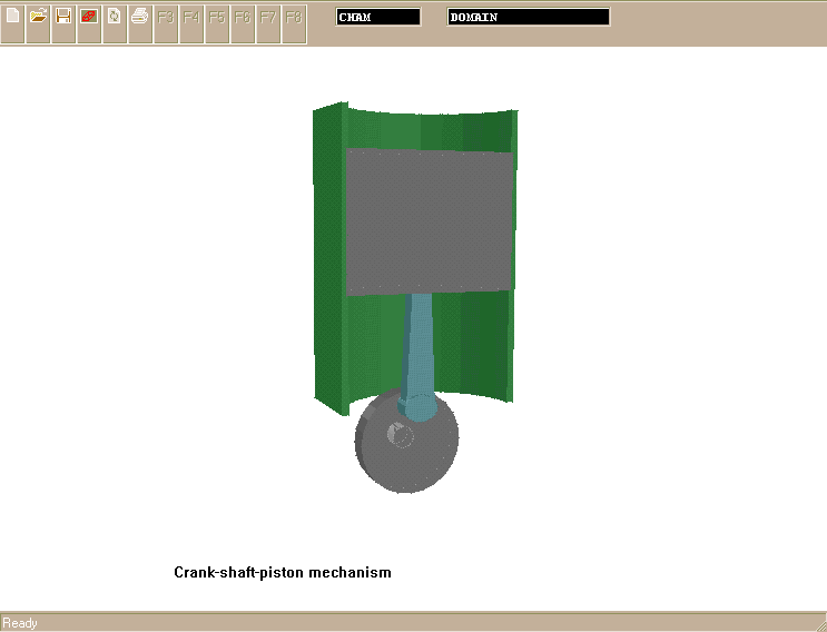
A mechanical example is the crank/connecting-rod/piston trio.
A human being, whose limbs are connected at joints (elbow, knee, etc) is also articulated.
It is this connectedness that the MOF format expresses by way of a hierarchy, whereby:
The MOF data file which describes a set of connected objects therefore has to convey information about the hierarchy (what is connected to what) and about the offset of each dependent element (also called "child") from its next-superior in the hierarchy (also called "parent").
It also indicates in what way each object can move.
Finally it states, for a succession of times, what have been the movements in each of the degrees of freedom.
A further explanation of the file is supplied here.
Alternatively, the information is supplied to the same locations by way of In-Form formulae, expressed via SPEDATs and conveyed via EARDAT.
It should be clearly understood that the time steps used in the CFD calculation are not necessarily the same as those in the MOF description. They may be larger or smaller.
This is performed by introducing appropriate momentum sources at the relevant nodes.
The necessary coding for this exists inside EARTH. It requires no user intervention.
if its boundaries are open (as when a grid which is fixed relative to a tennis-ball travels with it through the air),
then its motion must be expressed by suitable in-flow and out-flow sources at the grid boundaries.
If the computational grid is in accelerating motion, as when it is constrained to follow an accelerating rocket, so as to simulate the launch aerodynamics closely, the effect must be simulated by supplying corresponding 'body forces' at all velocity cells which lie within the fluid.
The necessary coding is provided in EARTH.
The values of the velocity and acceleration pertaining to each time
instant and each time interval are obtained by differentiation of
the position- and rotation-data contained in the MOF-data store in EARTH.
When scalar variables such as temperature or concentration are being solved, it is necessary to introduce further sources and sinks into the relevant finite-volume equations.
What needs to be done is readily recognised by consideration of the rectilinear motion of a heated but non-conducting solid which pushes colder non-conducting fluid ahead of it and is followed by a plug of the same fluid.
Obviously, the temperature profiles at two successive times ought to be as shown here:
       -------------               -------------
       |           |               |           |
       |           |               |           |  direction
       |           |               |           |  ----------->
       | earlier   |               |  later    |  of movement
       |           |               |           |
--------           -----------------           -------
Profiles approximating to these will be produced by PHOENICS if the
built-in temperature-solution procedure is activated; but smearing will occur,
by reason of 'false diffusion'; and, when specific heats are
not uniform, conservation of energy is not assured.
To achieve what is required, appropriate corrections to the finite-volume
equations must be made, in order to enforce correctness.
Click here to learn about the MOFOR cases in the Input-File Library.
Inspection of library case v112.htm as an example will show:
There is thus very little which needs to be placed in the Q1 file to
initiate a MOFOR calculation.
The MOF file associated with the just-examined Q1 is to be seen here
Its connexion with the Q1 is made by the presence in it of the words " BLOCK" and "TIP".
The "MOTION" table, at the bottom of the file, shows only two positions, for the beginning and the end; it is the value of LSTEP set by PHOENICS which breaks the time into 20 intervals.
It may be observed that both the degrees of freedom (i.e. "channels")
are rotations.
The facetdat file associated with the above example is shown here.
Inspection shows that it corresponds to the initial position of the objects.
Its use for mofor has therefore involved no enlargement or complication.
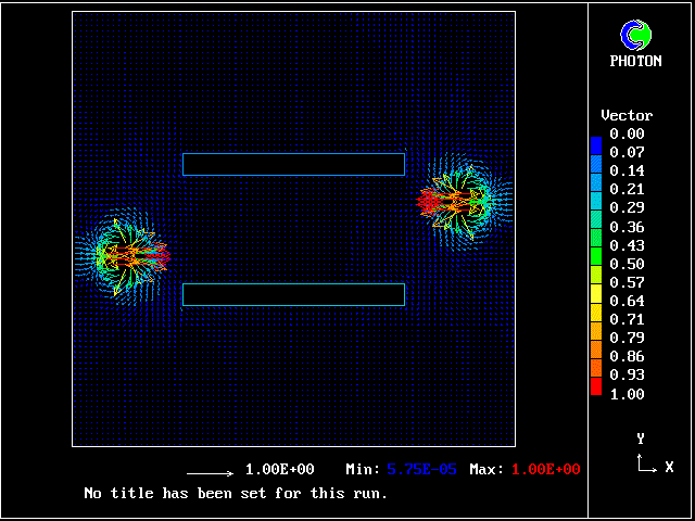
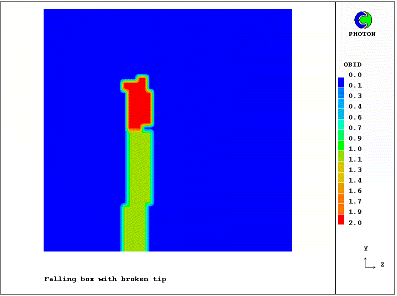
An animated PHOTON display of the results of the computation can be seen here.
Contours of OBID, the object identifier, are used for showing where the two moving objects are at each instant.
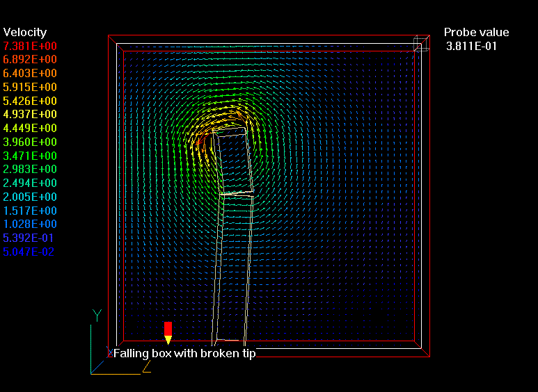
A second animation, in which the VR-Viewer is the displaying medium, is shown here.
This shows the boundaries of the box more correctly.
Since the 'macro-using' feature of Viewer is rather new, it is worth mentioning
that it uses precisely the same "use-file" commands as does PHOTON.
In order to enable PHOENICS users quickly to learn how to use MOFOR, a set of tutorials has been provided.
They can be accessed by clicking
here and
here
As mentioned above, further steps must be taken to ensure energy conservation in MOFOR.
No difficulties of principle are foreseen; but there exist many combinations of circumstance to be provided for.
Careful planning is therefore needed.
The situation is similar to, but perhaps easier than, that for thermal effects: no difficulties of principle; but careful planning and testing are needed.
Many exemplifications are needed, not just to test the method but also to convey
to PHOENICS users what a large number of applications can be made.
In order to be able to couple the motion of the body with the forces upon it, the latter must first be accurately calculated. This is not difficult in principle, because PHOENICS always does calculate the momentum balances on each cell.
The task is therefore one of using correctly information which is already available rather than that of starting anew.
A brief indication of what must be done is hinted at below:
Until now, the development work on PARSOL, which has involved almost complete re-writing, has been kept separate from that on MOFOR.
Now, however, both have advanced sufficiently for merging to be desirable and possible.
It is envisaged that, for handling the fluid-dynamical and thermal effects of moving bodies more accurately, use will be made of the volume and area "porosities ", which have been available from the earliest days of PHOENICS, but which were disregarded by PARSOL.
The merged coding for the faceted bodies will therefore compute these
quantities, as is indeed already done for In-Form-described bodies.
CHAM regards the work done so far as having confirmed the feasibility and economy of the MOFOR approach to the simulation of moving bodies.
It is certainly much simpler in concept and easier to implement than the approaches of other CFD-code vendors, who modify the grid at every time step, so as to accommodate the moving body.
Of course, simplicity and economy are not the only criteria; realism of the predictions is another.
It will therefore be a major objective of CHAM's further development program to test, and where necessary improve, the quality of the predictions made by MOFOR.
A familiar example is the 'sloshing' of a layer of liquid in a tank which is jolted, tilted, or caused to oscillate.
Such motions can also be handled by MOFOR, as illustrated by the following file fragments, namely:
Let it first be supposed that there exists a large fluid volume at rest, and that, within it there is present a computational grid which is in motion.
Let this motion be, in the first instance rectilinear, and such that the coordinates in absolute space of the origin of the grid, are expressible as known functions of time thus: xO(t), yO(y), zO(t).
Since PHOENICS employs finite time steps, Dt, say, the question arises of how xO' and xO'' are to be evaluated; and the answer is not obvious because, for example:
The correct answer is: the choices must be such as produce the exact solution described above; which is to say that the must accord with the choices adopted in the finite-volume formulations within PHOENICS.
Trial-and-error may well be the best mode of investigation.
Then the pressure within the grid will not remain constant in reality; and, if PHOENICS is properly solving the time-dependent equations of motion, the pressure variations which it predicts will be in accordance with reality.
Consider, for example, the case of a sphere of heavy material which, initially at rest relative to surrounding air, is suddenly released. Until its velocity increases sufficiently for the pressure and frictional forces exerted on it to be large (compared with the force of gravity), the sphere will fall at a velocity w,given by:
w = - g*t*, where g is the acceleration due to gravity and t is time.
Around the sphere, as time proceeds, a region of non-uniform pressure and velocity will be predicted; and the extent of this region will increase with time. However, until it extends to the outer boundaries of the grid, the above-mentioned velocity boundary conditions and within-grid body forces will suffice.
In the wake of the sphere, at the outlet boundary of the grid, the physically realistic velocity profile is certainly non-uniform. It would therefore be unrealistic to enforce the yO'(t) boundary condition there.
It is also unnecessary: a uniform-pressure boundary condition should suffice.
The built-in PARSOL procedures will represent the shape of the sphere adequately; and, because the grid and the object move together, the cut-cell calculation has to be performed only once.
The built-in forces-on-solid calculation procedure can be expected to function appropriately as all times. The magnitude of the calculated forces will increase in proportion to the third power of time; for it is proportional velocity squared; and velocity is proportional to time if the acceleration is constant.
g - F/sphere_mass ;
and, with the force F increasing (at first) in proportion to the t**3, it will soon fall to zero.
Therefore the acceleration must be calculated at each time step; then the velocity at the next time step can be calculated from it.
Once this deficiency is remedied, implementation should be quite straightforward.
It should be remarked that, for the falling-sphere problem, only one quarter of the whole domain needs to be simulated, because of the prevailing symmetries.
Three cases have been created to show how the 'moving-grid' method described above is applied to the simulation of moving objects with a constant acceleration and varying acceleration.
The first case simulates a sphere moving with a constant acceleration.
The velocity, U(t) used is a linear function of time
U(t)= t
Therefore the acceleration of the sphere is 1.0.
As required by the 'moving-grid' method described above, both at the boundaries of the grid, the velocities, must be given the prescribed values of U(t) at each time step; and within the volume the fluid must be subjected to accelerating forces of rho*1.0, per unit volume. Those are provided, by way of In-Form formulae as follows
patch(in,low,1,nx,1,ny,1,1,1,lstep)
(source of p1 at in is tim*rho1)
(source of w1 at in is tim with onlyms)
and
patch(acel,phasem,1,nx,1,ny,1,nz,1,lstep)
(source of w1 at acel is 1.0)
Complete settings and explanatory comments can be seen in the library case v207.
The Q1 file also contains a macro of commands which cause the Viewer when the macro button is pressed to display animation automatically.
It would be useful to check if the settings are consistent between the velocity boundary conditions and the acceleration-related body force by removing the sphere, so there is no object present within the domain. The calculation of this empty moving grid should show a uniform pressure and no pressure variation with time.
This case describes a sphere moving with varying acceleration.
For this case, a quadratic velocity function of time is used as follows
U(t) = t - t**2.0
where t is time
The acceleration is derived by the derivative of the velocity with respect to time as
accel = 1-2*t
The above velocity, U(t) is used, to provide, by way of In-Form formulae, boundary conditions for the mass flow and the velocity at the INLET as follows
patch(in,low,1,nx,1,ny,1,1,1,lstep)
(source of p1 at in is (tim-tim^2.0)*rho1)
(source of w1 at in is (tim-tim^2.0) with onlyms)
The above acceleration, accel is used to provide the domain body forces as follows
patch(acel,phasem,1,nx,1,ny,1,nz,1,lstep)
(source of w1 at acel is 1.-2*(tim-0.5*dt))
Note that 0.5*dt is to take the acceleration value at the middle of each time step.
Complete settings and explanatory comments can be seen in the library case v208.
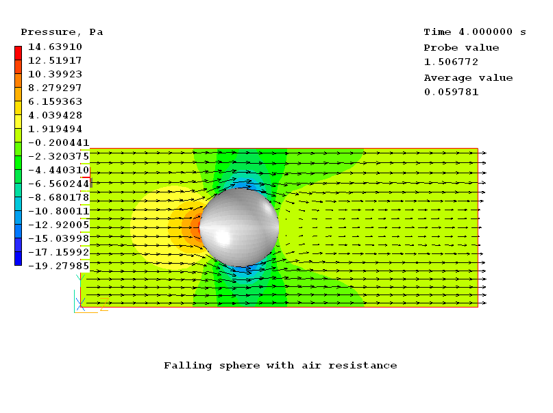
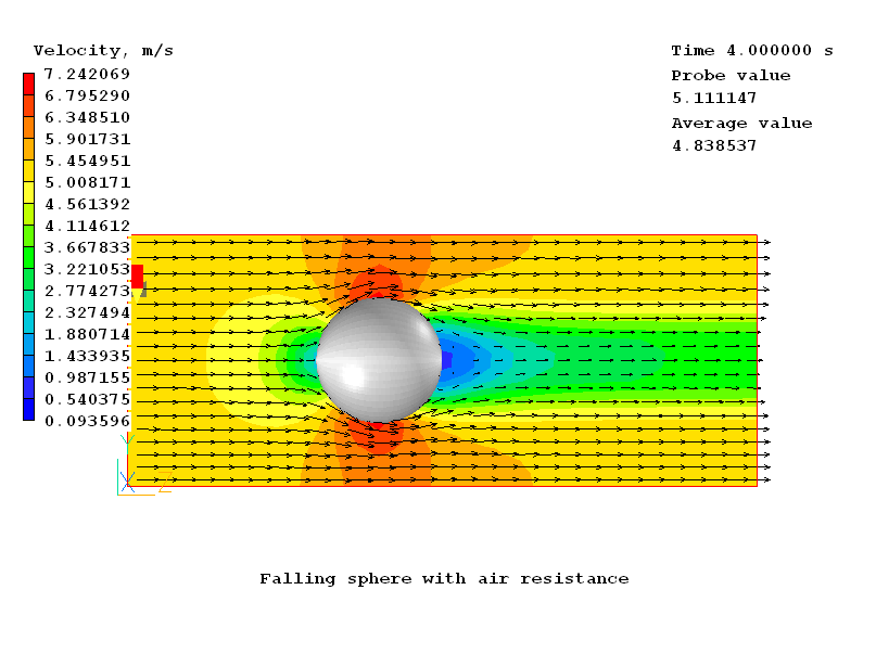
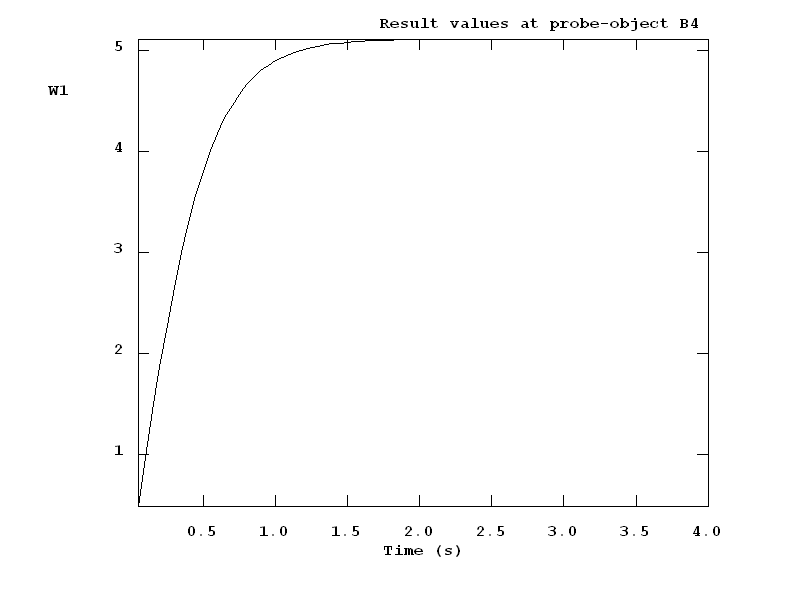
A sphere falling through air experiences a force in direction opposite to its motion. Terminal velocity is achieved when the drag force is equal in magnitude but opposite in direction to the gravity force propelling the sphere.
In this case, the quadratic drag equation is used to calculate the drag force as follows.
Fd = - 0.5 * rho * U**2.0 * A * Cd
where
The velocity of the sphere as a function of time can be derived as the following function:
U(t)= A1 * (EXP(A2*t)-1)/(EXP(A2*t)+1)
where
where
The acceleration, accel is given by the derivative of the velocity with respect to time , U(t)
accel = 4*A1**2.0*A3*EXP(A2*t)/(EXP(A2*t)+1)**2.0
where A3 is 0.5*rho*A*Cd/M
As for Case 1 and Case 2, the above velocity derived will be used to provide the boundary conditions for the mass flow (U*rho) and the velocity at the INLET, and the acceleration derived for the within-grid body forces.
In reality, the following terminal velcoty, Utm is asymptotically approached:
Utm = (2*M*G/rho*A*Cd)**0.5
which should also be obtained from the simulation if the calculation time is long enough.
The 'moving-grid' method is implemented by In-Form formulae written as follows.
SAVE13BEGIN
real(velin,aa1,aa2,aa3,aradi,vol1,area1,acd)
aradi=1.0
acd=1.0
area1=3.14159*aradi**2.0
vol1=4.0*3.14159*aradi**3/3.0
aa1=(2.0*9.81*vol1/area1/acd)**0.5
aa2=(2.0*9.81*area1*acd/vol1)**0.5
aa3=0.5*area1*acd/vol1
patch(in,low,1,nx,1,ny,1,1,1,lstep)
(source of p1 at in is :aa1:*(exp(:aa2:*tim)-1)/(exp(:aa2:*tim)+1)*rho1)
(source of w1 at in is :aa1:*(exp(:aa2:*tim)-1)/(exp(:aa2:*tim)+1) with onlyms)
patch(acel,phasem,1,nx,1,ny,1,nz,1,lstep)
(source of w1 at acel is 4*9.81*exp(:aa2:*(tim-0.025))/(exp(:aa2:*(tim-0.025))+1)^2.0)
(stored var E1 is 4*9.81*exp(:aa2:*(tim-0.025))/(exp(:aa2:*(tim-0.025))+1)^2.0)
SAVE13END
Complete settings and explanatory comments can be seen in the library case v209.
The Q1 file also contains a macro of commands which cause the Viewer when the macro button is pressed to display animation automatically.
Results
Four plots from the calculation are provided below
Plot 1 shows the pressure contours at time= 4s
Plot 2 shows the velocity contours at time=4s
The following picture shows the velocity varying with time and the terminal velocity of 5.11 m/s is approached when time reached 2.0 s
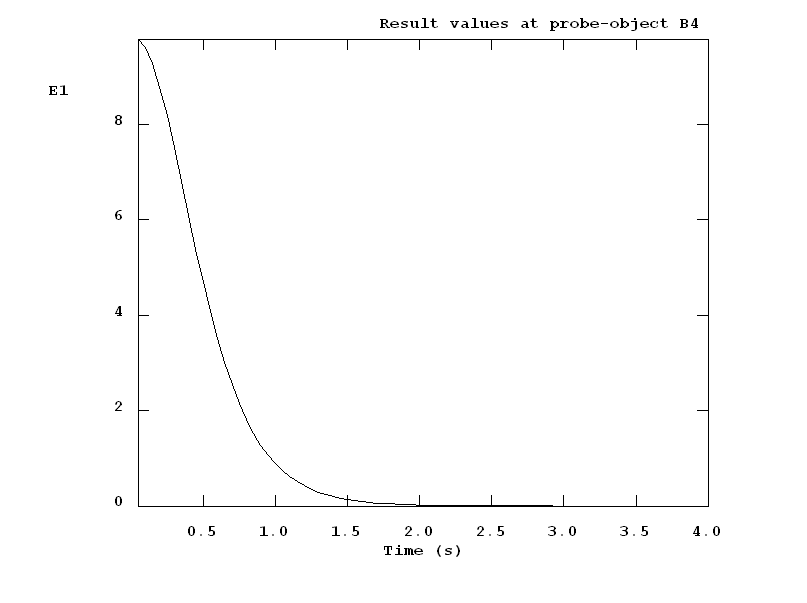
The following picture shows the acceleration (E1) of the sphere varying with time.