infrmobj.htm

Encyclopaedia Index

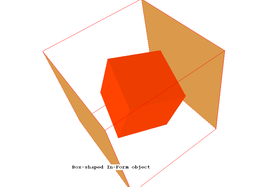
2.4 In-Form objects

Contents

Definition
Cell-enclosing (i.e. volumetric) shapes; box, sphere, ellipsoid
Cell-cutting (i.e. sub-grid) shapes; point, line, plane
Shapes made by restricting the PATCH size
Shapes made by using non-constant parameters
Shapes made by adding and subtracting
'Negative' objects
Positions varying with time
Shapes varying with time

(a) Definition

Two kinds of object

VR objects
- Since the introduction in 1995 of the 'Virtual-Reality' user interface, PHOENICS has made extensive use of 'objects'. [Click here for the relevant Encyclopaedia entry].
- Their shapes have been described by way of files, with .dat extensions, which define the locations of the vertices of the facets of which their surfaces are composed.
- Their positions, together with problem-specific re-sizings and re-orientations, have been conveyed to the PHOENICS solver-module EARTH by way of the file named FACETDAT.
- They will be referred to as Virtual-Reality objects below.
In-Form objects
- Now, indeed since 2004, In-Form allows the introduction of objects of its own kind. Their existence is inferred from the q1 file by the VR-Editor and-Viewer, and displayed, as shown by the following images.
  
  Their positions and shapes are marked:
  - first directly by geometric (i.e. x-y z) parameters, and then
  - indirectly by the indices of the cells which they enclose or penetrate.
- The specification of the geometric parameters is provided by formulae in the Q1 file; and it is conveyed to the solver by way of SPEDAT lines in the EARDAT file.
Similarities and differences between the two kinds of object are:
- Like Virtual-Reality objects, In-Form objects can be used for defining the locations of cells in into which initial values and sources are to be introduced.
- Both kinds of objects may change their positions with time; but only In-Form objects can also change their shape.
- However, whereas VR-objects are easily brought into a simulation scenario, and then located and resized by means of the menus and dialog boxes of the VR-Editor, this is not yet (March 2009) possible for In-Form objects.
- If any cell is occupied by two or more VR objects, only those initial values and sources which pertain to the object which appears last in the Q1 file are transmitted to that cell.
  For In-Form objects, this is true in respect of initial values also; but the sources are added together.
  In this respect they are similar to PIL PATCHes and dissimilar from VR objects.
- Moreover, because the information about In-Form objects is processed in EARTH later than that concerning VR objects, and without checking what has gone before, In-Form objects can be said to prevail over VR objects whenever both claim ownership of the same cell.
  Of course, since all In-Form formulae can be supplied with 'with (if(...))' conditions, checking can be enforced, if desired.
- Another point of difference is that whereas VR objects can be used for setting material properties only by way of initial values, In-Form objects allow such properties to be set via formulae which call for changes in response to varying pressure, temperature and other variables.
- Lastly, VR objects can be used for activating the PARSOL treatment of the 'cut cells' which its presence creates.
  With one exception (viz.the plane-quadrilateral), In-Form objects can not be so used at the present time.
  They can be used however for computing the volume and area porosities of the cells which they affect.
Work is in progress which should enable all appropriate In-Form objects to activate PARSOL by the end of 2011.

How In-Form objects are defined

In-Form objects are created and defined by means of statements of the following format:

(INFOB at PATCHNAME is FORMULA with infob_OBJNAME!options)

Here:

'INFOB' is a keyword, like 'PROPERTY', 'STORED' and 'SOURCE', which indicates what kind of information is to follow.
'PATCHNAME' is the user-chosen name in a PIL PATCH statement, which defines the 4-dimensional block of space-time within which the object is (or parts of it are) somewhere to be found;
The PATCH statement must be placed higher in the Q1 file than the INFOB statement referring to it.
'FORMULA' is a character string which defines the shape and position of the object in space and time. It may contain functions, like any other In-Form formula; but some functions (BOX, SPHERE, and others described below) are significant for In-Form objects alone.
'OBJNAME' is the user-chosen name (of which only the first 8 characters are significant) of the object.
'options' refers to any other of the conditions listed in Appendix 3 of the In-Form documentation; but one option, viz. PORO, has significance for In-Form objects only.

Two kinds of PATCH

Until April 2009, the space-time location of PIL PATCHes was almost invariably defined by way of the indices IXF, IXL, IYF, IYL, IZF, IZL, ITF, and ITL.

Partly because this conflicted in style with the grid-independent setting of In-Form objects, a new kind of patch, the so-called 'dot-patch' has now been introduced.

This sets the location by way of real-number arguments: RXF, RXL, RYF, RYL, RZF, RZL, RTF, and RTL. These represent the geometric coordinates, normalised by reference to XULAST, YVLAST, ZWLAST and TLAST, of the eight faces of the space-time block within the In-Form object is to be found.

Such patches, which are marked by having a dot, ., as the first character of their names retain their positions when the grid is changed.

It is for this reason that the use of dot-patches is to be preferred ot those of the old indicial type.

How In-Form objects are used

In-Form objects can be used for setting initial values, properties and sources by means of statements such as:


(INITIAL of PRPS at PATCHNAME is 67. with infob_OBJNAME)
(PROPERTY of RHO1 at PATCHNAME is 1.e-5*(P1+:PRESS0:) with infob_OBJNAME)
(SOURCE of TEM1 at PATCHNAME is xg+yg with infob_OBJNAME)

Thus the specific name of the object appears as an 'option' i.e. a 'modifier' of the source statement, Without it, the source would appear in all the cells of the patch.

It is however not necessarily the only one. For example, the above line could be modified to:

(SOURCE of TEM1 at PATCHNAME is xg+yg with infob_OBJNAME!fixval)

(SOURCE of TEM1 at PATCHNAME is xg+yg with infob_OBJNAME!fixflu)

If no additional option is added, the default !fixflu is presumed.

Currently available object shapes

At the present time (April 2009), six basic shapes of In-Form objects, and of two kinds, are provided, namely:

Cell-enclosing (also called 'volumetric') shapes, namely:
1. BOX,
2. SPHERE, and
3. ELLIPSOID,
and
cell-penetrating (also called 'sub-grid') shapes, namely:
1. POINT,
2. LINE, and
3. PLANE QUADRILATERAL.

However, objects of much more complex shapes may be constructed by using one or more of the following techniques:

restricting the dimensions of the PATCH so that parts of the specified shape lie outside it;
setting the arguments of the basic-shape functions (to be described) as expressions rather than constants; and
by 'adding' and 'subtracting' several basic shapes.

Further, the 'subtraction' feature permits creation of 'negative' objects, i.e. those in which the object attributes are applied to those cells which the object does not enclose or penetrate rather than to those which it does.

(b) The basic cell-enclosing (i.e. volumetric) shapes

Each of the basic shapes of the first group is described by an In-Form function possessing (nearly) the same name as the shape (but ELLIPSOID is shortened to ELLPSD). They will now be described, in turn.

The BOX function

The format governing the use of BOX in INFOB statements is indicated by the following example:
(INFOB at BOXPAT1 is BOX(arguments) with INFOB_BOX1)
where BOXPAT1 and BOX1 are names chosen freely by the user.

The arguments in question are as follows:
BOX(x0,y0,z0,xsize,ysize,zsize,alpha,beta,theta)
where
x0 = X-coordinate of west south low corner of box, in meters
y0 = Y-coordinate of west south low corner of box, in meters
z0 = Z-coordinate of west south low corner of box, in meters
xsize = X-size of box side, in meters
ysize = Y-size of box side, in meters
zsize = Z-size of box side, in meters
alpha = angle rotating around x axis, in radians
beta = angle rotating around y axis, in radians
theta = angle rotating around z axis, in radians

The six position and size arguments correspond to those which are used for VR-objects; but the three rotation arguments follow a different convention.

Library case 383 illustrates the use of the box function for the creation of a box in a cubical domain, with all its rotations equal to 0.25 radians, by means of the following statements:

  inform11begin
(stored of mark at patch1 is 1.0 with infob_1) ! MARK object
(initial of prps is 100 with infob_1) ! initialise PRPS
real(x0,y0,z0,xs,ys,zs,al,be,th)      ! declarations
x0=xulast/4   !  x/y/z position of box
y0=yvlast/4   !
z0=zwlast/4   !
xs=xulast/2   !  x/y/z size of box
ys=yvlast/2   !
zs=zwlast/2   !
al=0.25       !  alpha/beta/theta angles of coordinate system
be=0.25       !  of box
th=0.25       !
(infob at patch1 is box(x0,y0,z0,xs,ys,zs,al,be,th) with infob_1)  
  inform11end

Here, in order to make its shape and position visible in PHOTON and the VR VIEWER, the variable MARK has been stored and given the value of 1.0 for all the cells enclosed by the object.

It will be noticed that the often-convenient device is adopted of defining x0, y0, etc as real variables, and setting their values in statements which precede (INFOB ... .

In this case, the values are constants, which would not be difficult to read if inserted directly as:
BOX(:xulast/4:,:yvlast/4:, etc) ;
but, were they long formulae, their appearance following BOX( would make the line tiresomely long.

A PHOTON plot of the case-383 BOX object is shown here. It was created by the sur mark x 0.99 and sur mark y 0.99 commands.

In this example, each parameter is a constant; but each could have been a function, as will be illustrated in section (e) below.

The SPHERE function

The format governing the use of SPHERE in INFOB statements is similar to that of BOX, namely:
(INFOB at SPHPAT1 is SPHERE(arguments) with INFOB_SPH1)
where SPHPAT1 and SPH1 are names arbitrarily chosen by the user.

It has only four arguments however, namely:
SPHERE(xc, yc, zc, radius)
where
xc = x coordinate of the centre, in meters
yc = y coordinate of the centre, in meters
zc = z coordinate of the centre, in meters
radius = radius of the sphere, in meters
because rotations about its centre cannot change its shape.

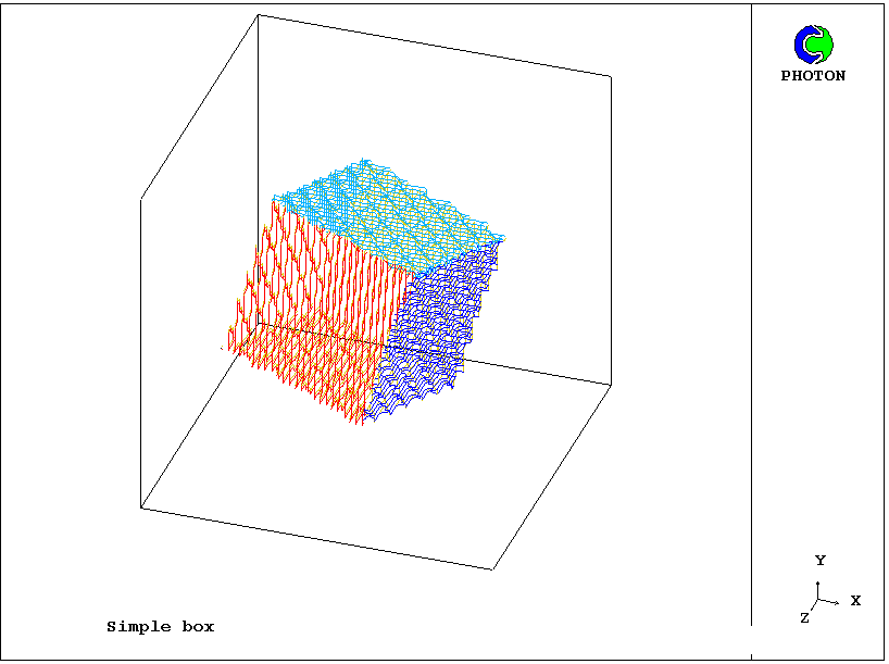
When the calculation is being carried out with a Cartesian grid, the coordinate system of the sphere coincides with the coordinate system of the calculation domain.

However, when the calculation is being carried out with a cylindrical-polar-coordinate grid, the cartesian coordinate system of the sphere has its origin at the bottom left-hand corner of a rectangular box which circumscribes a cylinder of radius RINNER+YVLAST.
In this case, cartesian coordinates xc and yc are related to the polar coordinates xp and yp by the relations:

xc=(yvlast+rinner) + (yp + rinner) * sin(xp)
and
yc=(yvlast+rinner) + (yp + rinner) * cos(xp)

The Z coordinates of the origins and the directions of Z axes of both coordinate systems coincide with one another.

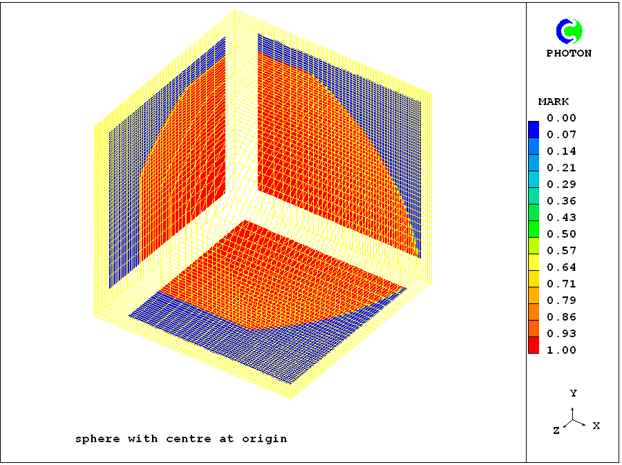
Library case 772 creates an In-Form object, namely a sphere with its centre on the axis of a polar grid, by means of:
(INFOB at PATCH1 is SPHERE(10, 10, 10, 5) with INFOB_1)

The PHOTON plot displayed here reveals the result.

In this case, it may be noted, xce, yce and zce are declared as character variables. This is the preferable procedure when the possible use of formulae as arguments is to be provided for.

The ELIPSOID function

The format governing the use of ELLIPSOID in INFOB statements is indicated by the following example:
(INFOB at ELLPAT1 is ELLPSD(arguments) with INFOB_ELL1)
where ELLPAT1 and ELL1 are names chosen freely by the user.

The arguments in question are as follows:
ELLPSD(x0,y0,z0,xrad,yrad,zrad,alpha,beta,theta)
where
x0 = X-coordinate of the centre of the ellipsoid, in meters
y0 = Y-coordinate of the centre of the ellipsoid, in meters
z0 = Z-coordinate of the centre of the ellipsoid, in meters
xrad = X-direction radius, in meters
yrad = Y-direction radius, in meters
zrad = Z-direction radius, in meters
alpha = angle rotating around x axis, in radians
beta = angle rotating around y axis, in radians
theta = angle rotating around z axis, in radians

Library case 384 illustrates the use of the ELLPSD function for the creation of an ellipsoid in a cubical domain, with all its rotations equal to 0.25 radians, by means of the following statements:

  inform11begin
(stored of mark at patch1 is 1.0 with infob_1) ! MARK object
(initial of prps is 100 with infob_1) ! initialise PRPS
real(x0,y0,z0,xs,ys,zs,al,be,th)      ! declarations
x0=xulast/4   !  x/y/z position of ellipsoid
y0=yvlast/4   !
z0=zwlast/4   !
xs=xulast/2   !  x/y/z radius of ellipsoid
ys=yvlast/3   !
zs=zwlast/4   !
al=0.25       !  alpha/beta/theta angles of coordinate system
be=0.25       !  of ellipsoid
th=0.25       !
(infob at patch1 is ellpsd(x0,y0,z0,xs,ys,zs,al,be,th) with infob_1)  
  inform11end

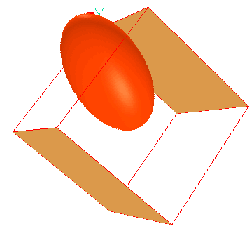
An image representing the ellipsoid created by core-input-file-library case 384 can be seen by clicking here.

Another example of the use of ellipsoid objects is core-library case 162, wherein the ellipsoid is given such an extremely large y-direction radius that, within the domain of study, it can be regarded as a cylinder.

It is indeed used there to represent a cylindrical pipe with an aperture in its walls from which gas is released into the atmosphere,

A fuller description of the situation can be found by clicking here,

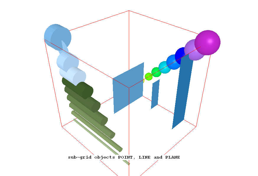
(c) The basic cell-cutting (i.e. sub-grid) shapes

Sub-grid objects are those of which one of the dimensions is smaller than that of the computational grid.

The three basic shapes of this kind are: POINT, LINE and PLANE; and to each there corresponds an In-Form function.

The POINT function

The format governing the use of POINT in INFOB statements is indicated by the following example:

(INFOB at PNTPAT1 is POINT(arguments) with INFOB_PNT1!options

where PNTPAT1 and PNT1 are names chosen freely by the user.

The arguments in question are as follows:
POINT(x0,y0,z0,nomdiam)
where:

x0 = X-coordinate of the point, in meters,
y0 = Y-coordinate of the point, in meters,
z0 = Z-coordinate of the point, in meters,
nomdiam = nominal diameter of the point.

The setting of point objects is exemplified in Core Library case 385, as seen by clicking here.

The LINE function

The format governing the use of Line in INFOB statements is indicated by the following example:

(INFOB at LINPAT1 is POINT(arguments) with INFOB_LIN1!optionsV

where LINPAT1 and LIN1 are names chosen freely by the user.

The arguments in question are as follows:
LINE(x0,y0,z0,x1,y1,z1,nomdiam)
where:

x0 = X-coordinate of the start point, in meters,
y0 = Y-coordinate of the start point, in meters,
z0 = Z-coordinate of the start point, in meters,
x1 = X-coordinate of the end point, in meters,
y1 = Y-coordinate of the end point, in meters,
z1 = Z-coordinate of the end point, in meters,
nomdiam = nominal diameter of the line.

The setting of line objects is exemplified in Core Library case 385, as seen by clicking here.

The PLANE function

The format governing the use of PLANE in INFOB statements is indicated by the following example:

(INFOB at PLAPAT1 is PLANE(arguments) with INFOB_PLA1!options)

where PLAPAT1 and PLA1 are names chosen freely by the user.

The arguments in question are as follows:
PLANE(
where:

x0 = X-coordinate of 1st vertex, in meters,
y0 = Y-coordinate of 1st vertex, in meters,
z0 = Z-coordinate of 1st vertex, in meters,
x1 = X-coordinate of 2nd vertex, in meters,
y1 = Y-coordinate of 2nd vertex, in meters,
z1 = Z-coordinate of 2nd vertex , in meters,
x2 = X-coordinate of 3rd vertex , in meters,
y2 = Y-coordinate of 3rd vertex, in meters,
z2 = Z-coordinate of 3rd vertex, in meters,
x3 = X-coordinate of 4th vertex, in meters,
y3 = Y-coordinate of 4th vertex, in meters,
z3 = Z-coordinate of 4th vertex, in meters,
nomdiam = nominal thickness of the plane.

Not all shapes are permissible, as shown here.

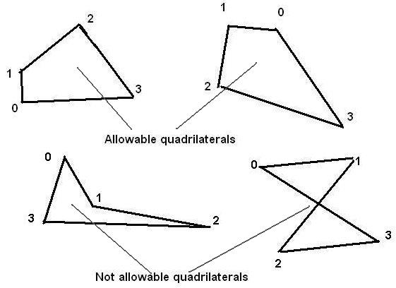
Further, if the user inadvertently selects four points which do not lie in a plane, the fact is detected by PHOENICS, which thereupon changes the 9th co-ordinate to such a value (there can be only one) which causes the fourth vertex to lie in the plane of the other three; or, if that is not possible, it does it for the 8th or the 7th.

It is sometimes useful to distinguish the two sides of the plane as being 'positive' or 'negative'. The convention adopted is that the positive side of the plane is that in which one must look if the first, second, third and fourth points are to apppear in clock-wise order.
Thus we are looking in the positive direction of the top-left quadrilateral above (and therefore seeing its negative side:
and we are looking in the negative direction at the top-right quadrilateral (and therefore seeing its positive side.

The setting of plane objects is exemplified in Core Library case 385, which employs PIL do loops to enable many objects to be set, in orderly groups

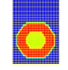
Graphical display

All the objects introduced in case 385 are displayed here by way of surface-value plots of PRPS which is specified as 100 within all the intersected cells.

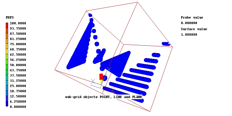
Points, lines and planes are all represented, the later by way of 'quadrilaterals' which have been reduced to triangles, as is always permissible, by having two cooincident vertices.

(d) Shapes made by restricting the PATCH size

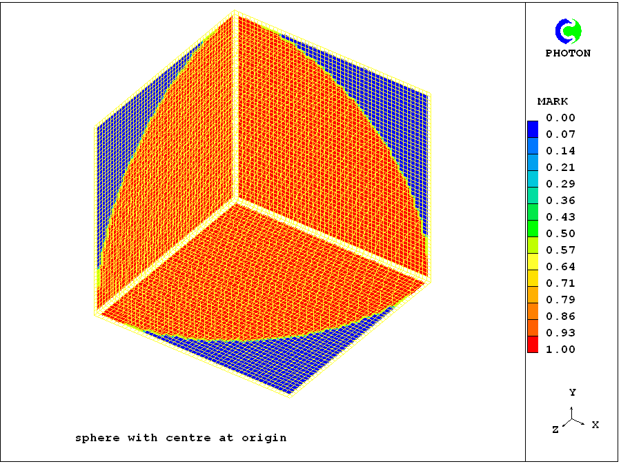
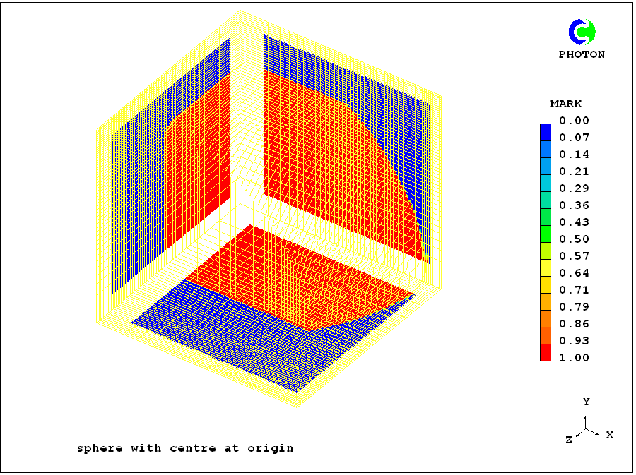
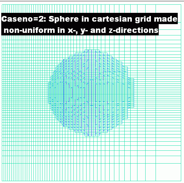
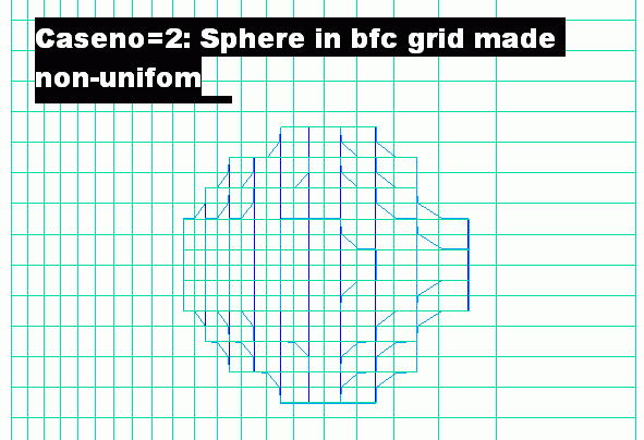
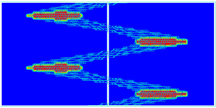
The sphere object

Core Input-File Library case 386 concerns a sphere placed in a cartesian grid with its centre at the co-ordinate axis. Its radius, and the domain dimensions, XULAST, YVLAST and ZWLAST, are all equal to 1m.

When the patch referred to in the INFOB command is as large as the whole domain, the photon picture showing the contours and surface of the MARK variable are as shown here.

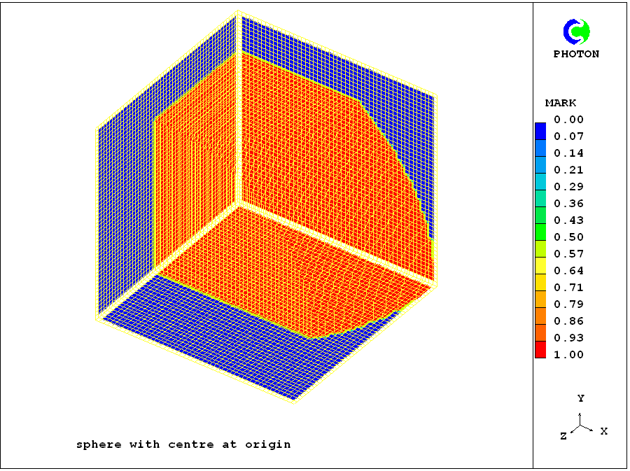
When the size of the patch is reduced by 20% and 40% respectively in the y- and z-directions, the corresponding images are those shown below, that on the left corresonding to use of an indicial patch and that on the right to a 'dot-patch'. They are of course identical.

When however the distribution of the grid intervals is drastically changed by making the fourth arguments of the GRDPWR statements 0.5 rather than 1.0, the corresponding pictures are as shown below:

Evidently the shape of the object has changed for the indicially-sized patch; but it has remained constant for the geometrically-sized one. That the grid change is the same in both cases is shown be the eqaual enlargement of the white bands used by PHOTON to high-light the co-ordinate axes.

Another example using spheres

Core Input-File Library case 785 illustrates the use of a size-restricting patch to confine two concentric spheres to the layer of cells adjacent to a domain boundary, where they are used so as to represent two apertures, one disk-shaped and the other annular.

Of the two images below, that on the left displays the shape of the apertures by way of MARK contours, while that on the right shows the associated velocity vectors.

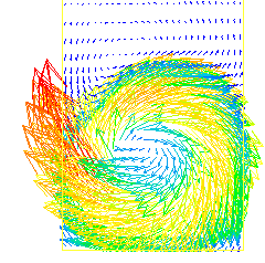
Of course, use of a finer grid would improve the circularity-appearance of the aperture edges. The use of a dot-patch makes this easy.

A final remark about the use of patches to limit object size

Although the just-demonstrated capability is sometimes useful, the fact that the surfaces of patches are by-definition aligned with the grid is a severe lmitation.

The use of 'subtraction', to be discussed in section (f) below, is much more powerful.

(e) Shapes made by using non-constant parameters

A pyramid made by use of the box function

Core input-file library case769 shows how, by using expressions rather than constants as arguments, the BOX function can be used for creating the pyramid shown below.

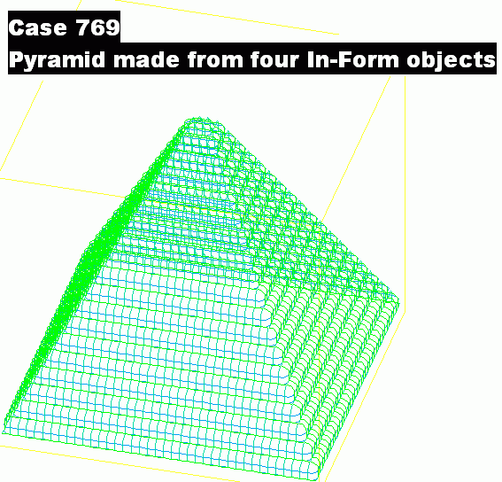
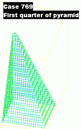
Examination of the Q1 file shows that the pyramid is composed of four parts, of which the first, created by the lines:

(INFOB at PATCH1 is BOX(10,10,0,.5*(-ZG+20),.5*(-ZG+20),$
16*(-ZG+20.),0,0,0) with INFOB_1!poros)

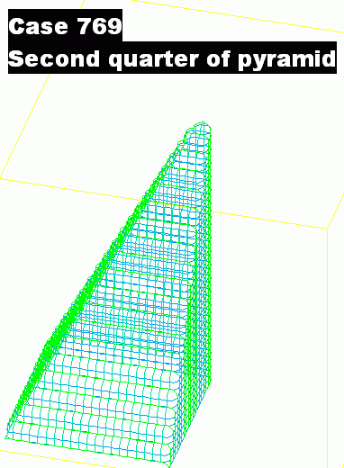
while the second is created by the lines:

(INFOB at PATCH1 is BOX(10,10,0,.5*(-ZG+20),.5*(-ZG+20),$
16*(-ZG+20.),0,0,.5*PI) with INFOB_1!poros)

in which the sole differences have been distinguished by the red font.

These first two quarters of the pyramid are shown below:

Let us now consider how it was that the quarter pyramids were created. The crucial steps were:

The two red-printed 'rotation' arguments above, and the two further ones which can be found for the third- and fourth-quarter statements,in the case-769 Q1, namely 3*PI/2 and 1.5*PI, dictated that the four quarters were each rotated by an extra right angle about the corner of the box at: x=10, y=10, z=0.
Then the first and second 'size' arguments, namely:
```
 5*(-ZG+20) and .5*(-ZG+20),
```
dictate that horizontal dimensions of the box diminish linearly as the height zG increases. This gives the object its 'pointed'shape.
The third 'size' argument, namely
```
16*(-ZG+20.)
```
proves to be much less important; indeed the person who introduced it was probably not perfectly clear as to what he or she was doing; for to insert
```
 ZG 
```
produces only porosity difference at the very peak of the pyramid; then inserting
```
 ZWLAST
```
or
```
2.0*ZWLAST
```
or any large-enough number produces no further differences at all!
All that is important is that, when the EARTH solver module is deciding about each cell having co-ordinates xG, yG and zG whether it lies inside of outside the box, the box appropriate to that cell should have a z-dimension large enough to enclose it.
Evidently, a truncated (i.e. flat-topped) pyramid could have been created by reducing the magnitude of the z-size argument.
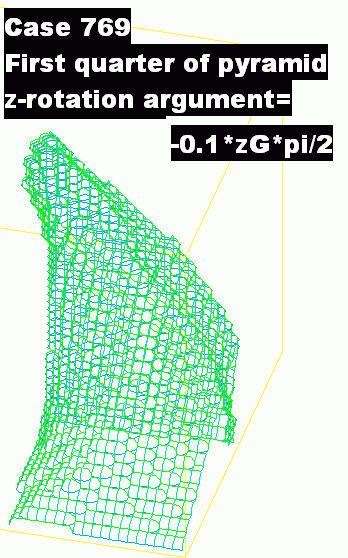
Now that the secret has been revealed, it is obvious that there is no limit to the variety of shapes which can be created. Here for example is a shape created by making the z-rotation argument decrease as zG increases:
Finally it should be mentioned that the four quarter-pyramids have all been given the same name, infob_1, in the case-769 q1. There is no objection to this; but, had it been desired to render display easier by giving each a diferent value of MARK, individual names would have been required.

Shapes made by use of the sphere function

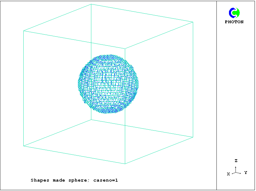
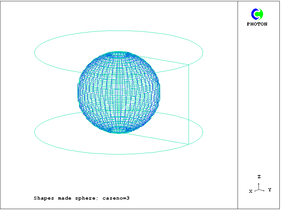
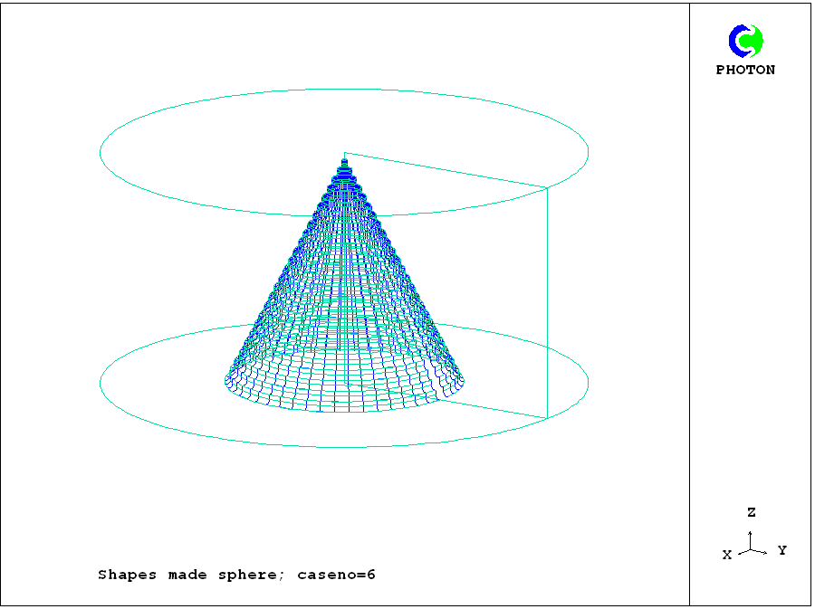
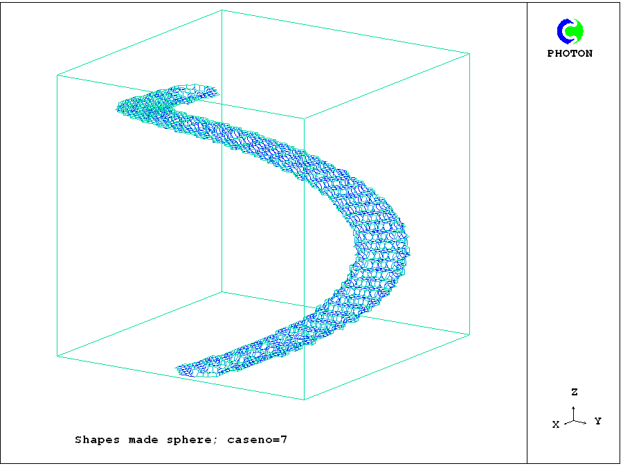
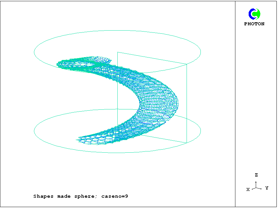
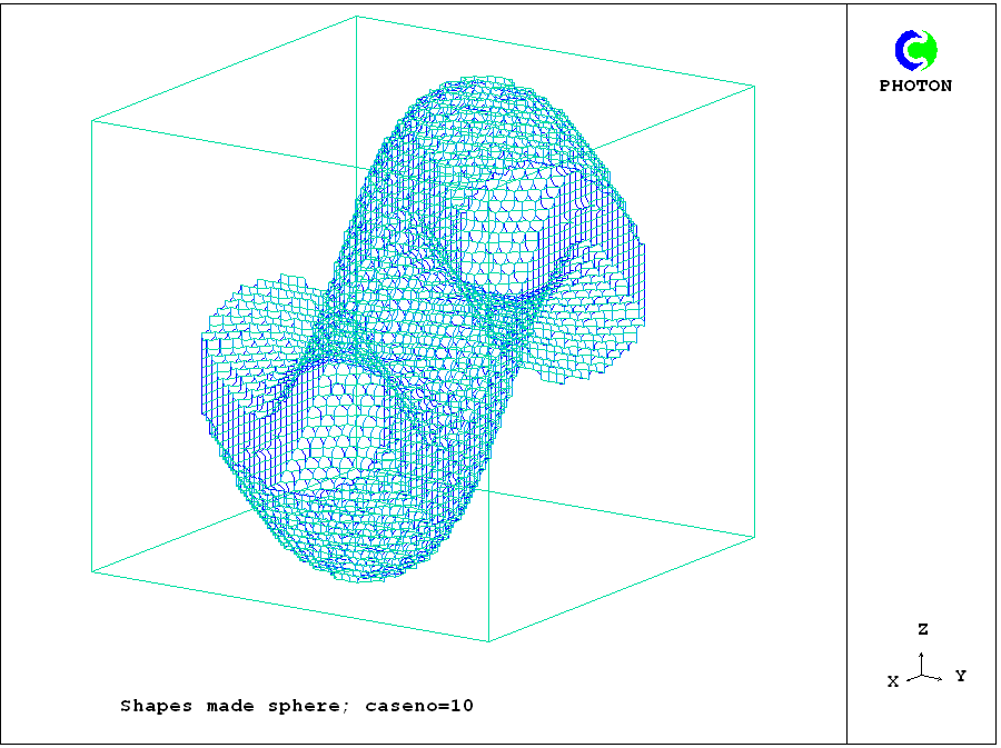
Core input-file library case749 shows how to create cones, spirals and a 'curved duct', by using the sphere object. It also enables tests to be made of the grid-independence of the In-Form-object settings.
Cartesian. cylindrical-polar and BFC grids are all represented.

The following hyperlinks lead to photon displays of the various shapes:

caseno shape grid type hyperlinks

1 fixed sphere cartesian click here

2 fixed sphere bfc click here
3 fixed sphere polar click here
4 cone cartesian click here
5 cone bfc click here
6 cone polar click here
7 spiral cartesian click here
8 spiral bfc click here
9 spiral polar click here
10 curved duct cartesian click here
11 curved duct bfc click here

caseno	shape	grid type	hyperlinks
1	fixed sphere	cartesian	click here
2	fixed sphere	bfc	click here
3	fixed sphere	polar	click here
4	cone	cartesian	click here
5	cone	bfc	click here
6	cone	polar	click here
7	spiral	cartesian	click here
8	spiral	bfc	click here
9	spiral	polar	click here
10	curved duct	cartesian	click here
11	curved duct	bfc	click here

In the following table are shown the values of the arguments of the sphere function in the infob statement for the various cases. namely:

(infob at .patch1 is sphere(x0,y0,z0,rad) with infob_1)

caseno x0 y0 z0 rad

1 xulast/2 yvlast/2 zwlast/2 xulast/4

2 xulast/2 yvlast/2 zwlast/2 xulast/4
3 xulast/2 yvlast/2 zwlast/2 yvlast/2
4 xulast/2 yvlast/2 zg 0.25*(:zwlast:-zg)
5 xulast/2 yvlast/2 zg 0.25*(:zwlast:-zg)
6 yvlast yvlast zg 0.5*(:zwlast:-zg)
7 :xulast/2:*(1+0.8*cos(:PI2:*zg)) :yvlast/2:*(1+0.8*sin(:PI2:*zg)) zg zwlast/10
8 :xulast/2:*(1+0.8*cos(:PI2:*zg)) :yvlast/2:*(1+0.8*sin(:PI2:*zg)) zg zwlast/10
9 :yvlast:*(1+2*:rad:*cos(:PI2:*zg)) :yvlast:*(1+2*:rad:*sin(:PI2:*zg)) zg yvlast/4
10 xg :yvlast/2: :zwlast/2:+0.25*sin(:pi2:*xg/xulast) yvlast/4
11 xg :yvlast/2: :zwlast/2:+0.25*sin(:pi2:*xg/xulast) yvlast/4

caseno	x0	y0	z0	rad
1	xulast/2	yvlast/2	zwlast/2	xulast/4
2	xulast/2	yvlast/2	zwlast/2	xulast/4
3	xulast/2	yvlast/2	zwlast/2	yvlast/2
4	xulast/2	yvlast/2	zg	0.25*(:zwlast:-zg)
5	xulast/2	yvlast/2	zg	0.25*(:zwlast:-zg)
6	yvlast	yvlast	zg	0.5*(:zwlast:-zg)
7	:xulast/2:(1+0.8cos(:PI2:*zg))	:yvlast/2:(1+0.8sin(:PI2:*zg))	zg	zwlast/10
8	:xulast/2:(1+0.8cos(:PI2:*zg))	:yvlast/2:(1+0.8sin(:PI2:*zg))	zg	zwlast/10
9	:yvlast:(1+2:rad:cos(:PI2:zg))	:yvlast:(1+2:rad:sin(:PI2:zg))	zg	yvlast/4
10	xg	:yvlast/2:	:zwlast/2:+0.25sin(:pi2:xg/xulast)	yvlast/4
11	xg	:yvlast/2:	:zwlast/2:+0.25sin(:pi2:xg/xulast)	yvlast/4

The following points should be noted:

The images and the arguments, are the same for both the cartesian and the body-fitted co-ordinate grids, as they should be, even though the handling of the geometry within the solver.
For the polar grid, the differences in the parameters consist in using yvlast rather than yvlast/2 to describe the horizontal dimension; and in avoiding the use of xulast, which ix now equal to 2*pi radians rather than 1 meter. x0, however, is still a distance in meters.
The cross-section of the spiral is not, as might have been expected, that of a circle of radius rad; instead it approximates to a flattened ellipse, only the horizontal dinesion of which is equal to 2*rad.
The flattening is greater the smaller is the axial distance between successive turns.
For example, what happens when the multiplier ofpi2 in the expressions for x0 and y0 of caseno=9 is zg*2 rather than zg is shown by this photon image:

The grid is not fine enough to show the shape well; but the flattening is unmistakeable.
Summarising, it can be said that although finer grids are needed if perfection is required, the independence of the type of grid has been demonstrated.

Library case 249 also possesses two boolean variables: altercrt and alterbfc. Both were set false in all the cases shown so far; but, when set true,the former alters the cartesian grid and the latter alters the bfc one. They have been used for further testing the grid-independence of the In-Form object settings, with the results shown here.

Clearly, although the distribution of the grid lines does affect the smoothness of its surface, the position of the sphere in cartesian space is not infuenced by it.

The bfc grid, it should be mentioned, was coarsened as well as distorted because the the execution of the PIL do loop in the Q1 file, by which the distortion was effected, is rather slow.

case 768 reveals that there is more than one way to create a spiral in a polar-coordinate grid; and its way of doiing so does create cross-sections which are more truly circular than those of case 749, as the next Photon image shows:

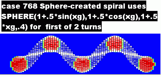
This method, as is seen, uses the angular coordinate xg in the formula; therefore it is necessary to use two spheres for the two-turn spiral shown here. They can however, if desired, be specified in a single INFOB statement, as is explained by comments in the Q1 file of the case.