W1

-----------------------------------------

Integer flag; value=7.

W1....standard name used to denote the first-phase velocity component in the iz-direction.

See PHI and NAME for further information.

W1AD

------ PIL real; default= 0.0; group 8 --- -

W1AD....add extra velocity W1AD to W1. See U1AD and ZMOVE.

When it is desired to use the z-wise moving-grid option, set W1AD= ZMOVE.

W2

-----------------------------------------

Integer flag; value=8.

W2....standard name used to denote the second-phase velocity component in the iz-direction.

See PHI and NAME for further information.

W2AD

------ PIL real; default= 0.0; group 8 --- -

W2AD....add extra velocity W2AD to W2. See U1AD.

W2CR

------ PIL character flag; group 7 --------

W2CR....integer name recognized by EARTH denoting second-phase cartesian ZC-directed velocity resolute. See UCRT.

WALDIS

WALDIS is an integer index, usable in subroutines called from GROUND, for accessing the 2D array of values, pertaining to the current IZ-slab, of: twice the distance from the wall to the first internal node. It is used in connection with the wall functions for turbulence models.

WALPRN

----- PIL logical; default=F; group 21 -- -

WALPRN....when set to T causes print-out of wall heat-transfer coefficients for patches created by a CONPOR command where the porosity factor is negative and wall friction has been activated, provided that the following conditions are also satisfied:

1. temperature is solved for, ie SOLUTN(TEM1,Y,Y...);
2. the flow must be turbulent, with SOLUTN(KE,Y,Y...);
3. if NZ is greater than 1, NPRINT must be set to LSWEEP-1.

WC1

------------ PIL integer flag

WC1.... name used to denote the first-phase co-located velocity component in the z-direction.

WCRT

------ PIL character flag; group 7 --------

WCRT....integer name recognized by EARTH denoting first-phase cartesian ZC-directed velocity resolute. See UCRT.

WEST

------ PIL real flag; value= 3.0; group 13 -

WEST....PATCH TYPE used for setting sources per unit west ( ie. smaller-x ) area by way of COVAL in group 13.

WGRDNZ

WGRDNZ is an integer index, usable in subroutines called from GROUND, for accessing the 2D array of values, pertaining to the current IZ-slab, of:
values of the w-velocity of the grid at the high face of each z-slab when the moving-grid option is active. The array is accessed via GETZ and holds values for all IZ. See W1AD or ZMOVE for more information on the moving grid option.

Wh.Field

----------------------------------- Photon Help ----

Streamlines will be tracked in the entire domain, both downstream and upstream of the starting positions.

WHEN

-------------- Advanced PIL command --- -

WHEN is the second element of the PIL CASE construct. See the HELP entry on CASE for further information.

WHERE

-------------------------------------- Photon Help ----

WH[ere].... is a REPLAY command which displays the graphics cursor, and returns the position when an alphanumeric key is pressed. It is used to find screen positions for text and frame positioning, for use with the USHIFT and UTEXT commands in USE files.

See also : REPLAY, USHIFT, UTEXT

Whole-field pressure corrections

(see PCOR integer name, Group 7)

Whole-field solution, definition of

'Whole-field solution' is a procedure which can be employed by PHOENICS for any variable. It reduces the number of sweeps which must be made in order to eliminate the imbalances in the equations; but it uses more computer storage and more time. Whole-field solution is most effective for phenomena such as 'pure' heat conduction, or irrotational (ie 'potential') fluid flow; for then a single sweep may suffice to give the solution.

Whole-field variables, number of

(see NPHI integer name, Group 7)

WIND, a PHOENICS-VR object type

A WIND object is used to specify the atmospheric boundary layer profiles at the edges of the domain, given a prevailing wind direction and speed. It performs several functions. It creates:

1. A WIND_PROFILE at the upwind faces of the domain;
2. An OUTLET at the downwind faces of the domain; and
3. An optional OUTLET at the sky boundary.

WIND_PROFILE, a PHOENICS-VR object type

Window

(Main graphics widow) ------------------------------------- Photon Help ----

[W]indow creates a new PHOTON window. There are a number of attributes attached to each window: view direction, up direction, magnification factor. The graphic elements created in a window will permanently belong to the window. With the default setting, a graphic element can only be redrawn in the window to which belongs . This can be changed by toggling the [S] in the window title bar to [A].

WRITE

------- PIL COMMAND

The WRITE command will write text to a new file, or append text to an existing file. The file could be a batch file which is to be executed with the the EXEC command.

To create a new file, use

WRITE(>filename,string1,string2,....,stringn)

To append to an existing file, use

WRITE(>>filename,string1,string2,....,stringn)

If the file filename does not exist it will be created. The file name may have spaces in it. If it does exist, it will be deleted and recreated for WRITE(> or appended to for WRITE(>>.

The strings string1, string2 may also contain spaces. Individual arguments are written to the output file separated by spaces. Thus

WRITE(>myfile.txt,Here is some,text)

will create the file myfile.txt containing the line

Here is some text

Note that a comma is used as a delimiter between arguments to WRITE. If it is required to include a comma as part of a string, it must be preceded by a |. To include a | in the string, use ||. For exampe, the command

WRITE(>myfile.txt,a|,b,c||d)

will create a file called myfile.txt with the contents

a,b c|d

See also the entry on character handling here to see how to preserve the case and spacing of text strings.

WSR (i.e. Well-stirred reactor)

Contents

1. 'Micro' and 'macro' WSRs
2. Extinction of combustion in a 'micro' WSR
3. Extinction in a 'macro' WSR, analysed by the MFM
4. Continuously varying attributes; NOX production

1. 'Micro' and 'macro' WSRs

PHOENICS is equipped to distinguish two kinds of WSR, namely:

1. the 'micro' (i.e. originally-conceived) WSR, in which the instantaneous temperature and concentrations of all species are identical for all locations within the reactor volume, and

2. the 'macro' WSR in which only the time-average temperature and concentrations of all species are identical for all locations within the reactor volume.

The distinction is important because flows in most practical reactions are turbulent. As a consequence, although sufficiently-vigorous stirring will bring a real reactor quite closely to the 'macro-WSR' state, attainment of the 'micro-WSR' state, in which even micro-scale non-uniformities are absent, is scarcely ever possible.

This is applies especially to combustion reactions, of the kind occurring in engines and furnaces, for which the rapid temperature-dependent reaction rates accentuate the local non-uniformities.

The 'macro WSR' is therefore by far the more realistic object of study.

The names of the models will be abbreviated to IWSR ( the I coming from Ideal or mIcro) and AWSR (the A coming from mAcro or Average) from now on. The following description exemplifies the AWSR idea. It is taken from MFM-library case L001.htm

  Stirred reactor with a 1D population distribution, and
  reactedness, ranging from zero to 1, as the population-
  distinguishing attribute.
                                                 ___________
  It is supposed that two streams of fluid      |           |
  enter a reactor which is sufficiently    A ====>          |
  well-stirred for space-wise differences       |  stirring |
  of conditions to be negligible, but not       |  \\\|/// C===>
  sufficiently for micro-mixing to be           |  paddle   |
  complete.                                B ====>          |
                                                |___________|
  The two entering streams have the same elemental
  composition; but one may be more reacted than the other.

2. Extinction of combustion in an IWSR

The analysis for IWSRs is the simpler, and will be presented first, for the case of a single entering stream of pre-mixed fuel and oxidant.

The following diagram from an old lecture forms the starting point. It shows the typical shape of the dependence of the rate of reaction on the 'reactedness', i.e. the extent to which reaction has progressed.

As indicated by the abscissa legend, reactedness can be measured, for an adiabatic system, by the dimensionless temperature rise, where Tu stands for the temperature of the fully-unburned gas and Tb for that of the fully-burned gas.

 __________________________________________________________________
 | combustion  |   11  | 2. The "simple chemically-reacting system"|
 | lecture     |  ---- |    (SCRS), 5:                             |
 |    1        |   20  |    Reaction rate for fixed f and h        |
 |_____________|_______|___________________________________________|
 |          |*      oxygen---> x               # #                 |
 |          |    *                x           #   #                |
 |          |        *               x       #     #               |
 |          |           *               x   #       #              |
 |          |               *              x         #<--reaction  |
 |          | unburned fuel---> *         #   x       #  rate, R   |
 |          |                       *   #        x     #           |
 |          |                         # *           x              |
 |          |                       #       *          x#          |
 |          |                     #             *         x        |
 |          |                  #                    *    #         |
 |          |           #                               *          |
 |          #---------------------------------------------#        |
 |          0    reactedness, r ( = (T - Tu)/(Tb - Tu) )  1        |
 |_________________________________________________________________|

• the rate increases rapidly with temperature, which explains the concave-upward shape of the left-hand part of the curve;
• it must fall to zero when the concentration of either of the reactants (fuel or oxidant) becomes zero; and
• this happens, as is shown by the two straight lines on the diagram, when the burned-gas temperature is reached.

Now let it be recalled that, in the steady state, two relations between r and R must be obeyed, namely that indicated above, and another which expresses the conservation of fuel mass, namely:

             Mdot * mfu,u * r =  R * vol
     where:        
             Mdot  = mass flow rate of the entering fuel-bearing stream,
             mfu,u = mass fraction of fuel in this stream, and
             vol   = reactor volume. 
             

 ___________________________________________________________________
 |          |                                  # #          +      |
 |          |                                 #   #     +          |
 |          |                                #     #+              |
 |          |                               #   +   #              |
 |          |  mass-balance line           #+        #>--reaction  |
 |          |                 \         + #           #  rate, R   |
 |          |                  \    +   #              #           |
 |          |                   +     #                            |
 |          |               +       #                   #          |
 |          |           +         #                                |
 |          |       +          #                         #         |
 |          |   +       #                                          |
 |          #---------------------------------------------#        |
 |          0    reactedness, r ( = (T - Tu)/(Tb - Tu) )  1        |
 |_________________________________________________________________|

When however the slope increases, for example by increase of mass flow rate, to a critical value, only one (low-temperature) intersection exists: combustion has been extinguished.

3. Extinction of combustion in an AWSR

However, since the the IWSR model takes no account of turbulent fluctuations, greater realism is to be expected from an AWSR analysis based on the 'multi-fluid model of turbulent combustion'.

An account of the general implications of such an analysis can be seen by clicking here.

PHOENICS Library case L103 enables the extinction phenomenon to be observed by variation of the quantity FLOWA, the mass-inflow rate.

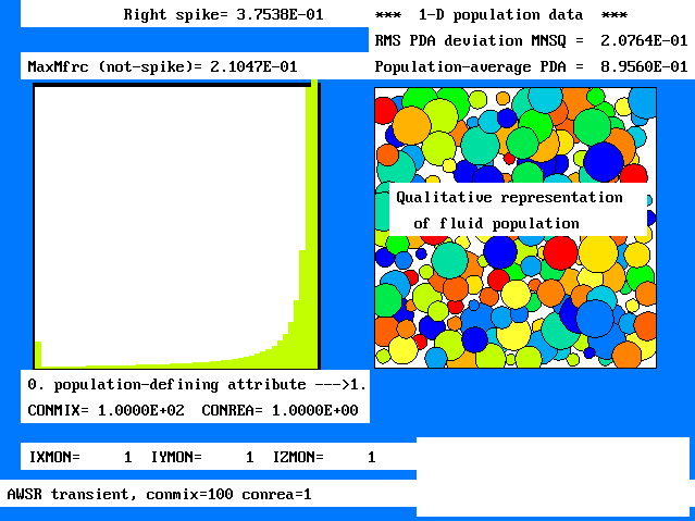
With the default value of 1.0 kg/s, the PDF for the steady state , which is achieved after less than 50 seconds, shows a 'spike' at reactedness 1.0 .

The following line-printer plot shows how the mass fractions of some of the fluids (curves 2, 3, 4 and 5) with time. Specifically, they all approach, asymptotically, finite values between 0.0 and 1.0(or 0.1), emplying that steady-state combustion takes place.

   Variable    1 = RCTD   2 = F44    3 = F46    4 = F48    5 = F50
     Minval=  0.000E+00  0.000E+00  0.000E+00  0.000E+00  0.000E+00
     Maxval=  1.000E+00  1.000E-01  1.000E-01  1.000E-01  1.000E+00
     Cellav=  9.745E-01  1.801E-02  3.045E-02  7.744E-02  4.381E-01
   Variable    6 = AVER
     Minval=  0.000E+00
     Maxval=  1.000E+00
     Cellav=  9.035E-01
 1.00 611111....+....+....+....+....+....+....+....+....+
      56666 1111111111111111111 1111111111111111111111111
 0.90 +5   66666666666666666666 6666666666666666666666666
      .             4444444                             .
 0.80 + 5        444                                    +
      .  5      4                                       .
 0.70 +        4                                        +
      .   5   4                                         .
 0.60 +    5 4                                          +
      .     5                                           .
 0.50 +      55                                         +
      .    4   55                                       .
 0.40 +          55555555555555 5555555555555555555555555
      .   4         33333333333 3333333333333333333333333
 0.30 +  4     33333                                    +
      .      33                                         .
 0.20 + 4  33   222222222222222 2222222222222222222222222
      .   3 2222                                        .
 0.10 +43322                                            +
      432                                               .
 0.00 3....+....+....+....+....+....+....+....+....+....+
      0   .1   .2   .3   .4   .5   .6   .7   .8   .9  1.0
 the abscissa is      ISTP.  min= 1.00E+00 max= 5.00E+01

 

• The first represents the reactedness which would be attained if the reactor were fully mixed at the micro-scale level, i.e. if the reactor were an IWSR.
• The second represents the population-average for the AWSR.

They do not coincide; and indeed the IWSR reactedness is much closer to unity than the AWSR reactedness.

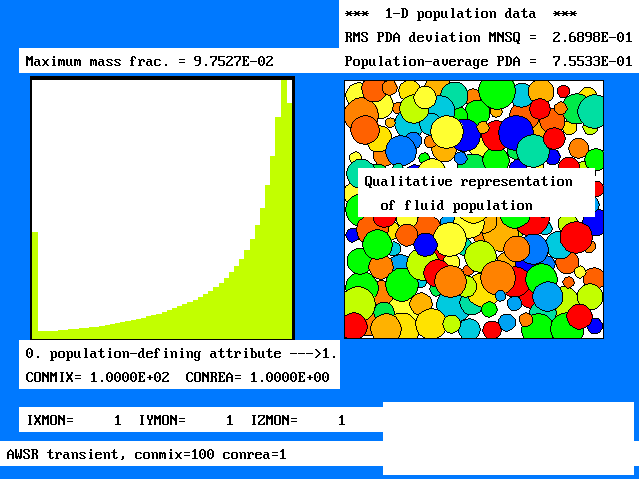
Doubling the mass-inflow rate changes the PDF to this, which lacks the right-hand spike, and has a much-lower population-average reactedness.

This is confirmed by the following time-wise line-printer plot:

 1.00 1....+....+....+....+....+....+....+....+....+....+
      6611111111111111111111111 1111111111111111111111111
 0.90 5 66     44444444444                              +
      .   666 4           44444 4444444444444444444444444
 0.80 +5     666666666                                  +
      .     4         666666666 6666666666666666666666666
 0.70 +    4                                            +
      . 5                                               .
 0.60 +   4                           3333333333333333333
      .  5         333333333333 333333                  .
 0.50 +         333                                     +
      .  45   33                            2222222222222
 0.40 +      3      22222222222 222222222222            +
      .    53   2222                                    .
 0.30 + 4 3 5 22                                        +
      .     255                                         .
 0.20 +  322   55                                       +
      .432       55555                                  .
 0.10 +32             555555555 5555555555555555555555555
      42                                                .
 0.00 2....+....+....+....+....+....+....+....+....+....+
      0   .1   .2   .3   .4   .5   .6   .7   .8   .9  1.0
 the abscissa is      ISTP.  min= 1.00E+00 max= 5.00E+01 

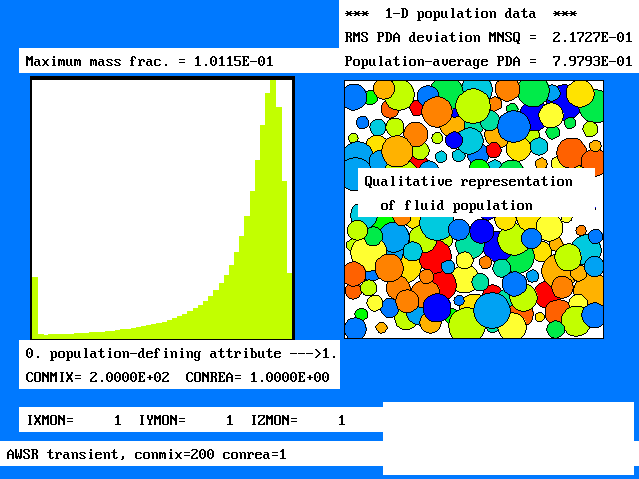
A further increase of flow rate, namely to 2.5 kg/s leads swiftly to extinction, as evidenced by this PDF, and the corresponding line-printer-plot:

 1.00 1....+....+....+....+....+....+....+....+....+....+
      611111111                                         .
 0.90 566      1111111111111111 1111111111111111111111111
      .  66                                             .
 0.80 +    6664444                                      +
      .5    4 666666                                    .
 0.70 +    4        66666666666 66666666                +
      .               444               66666666666666666
 0.60 + 5 4              444                            +
      .                     444 44                      .
 0.50 +  5     3333333333333333   444444                +
      .      33                 33333333444444444       .
 0.40 +   5 3     2222222222222 2222222222222233344444444
      . 4  3  2222                                      .
 0.30 +   3522                                          +
      .  3 25                                           .
 0.20 +4  2  55                                         +
      . 32     55                                       .
 0.10 +32        55555                                  +
      42              555555555 5555555555555555555555555
 0.00 +....+....+....+....+....+....+....+....+....+....+
      0   .1   .2   .3   .4   .5   .6   .7   .8   .9  1.0
 the abscissa is      ISTP.  min= 1.00E+00 max= 5.00E+01

For this flow rate, combustion could therefore survive in an ideal WSR, but not in the AWSR under study.

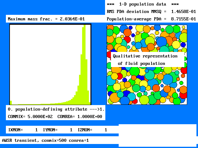
It is natural to ask: by how much would the stirring rate in the WSR have to be increased in order to prevent extinction?

This question can be answered by repeating the calculation with various values of MFM's 'mixing constant, CONMIX, which had the value 100.0 for the above calculations, implying a 'mixing time' of the order of 0.01 seconds.

A doubling of CONMIX proves to be (just) sufficient. It leads to the steady-state PDF shown here.

A five-fold increase of CONMIX has an even greater effect, as the corresponding PDF reveals. Indeed the population-average reactedness is approaching the value of 0.92, which was predicted for the IWSR.

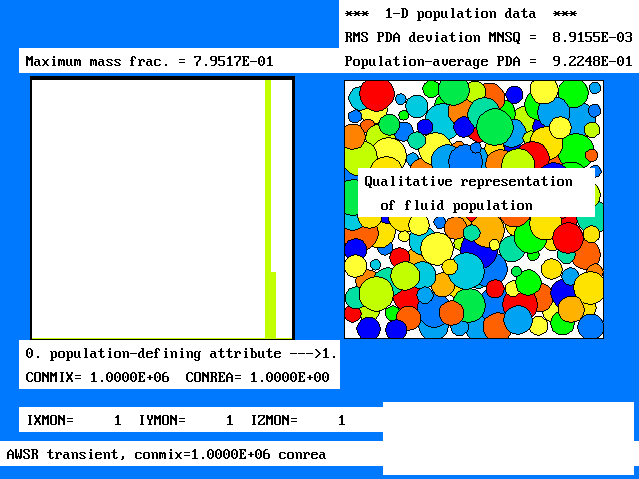
Of course, an immense increase of CONMIX, namely to 1.0E6, gives results which are even closer to those of the IWSR, as the next PDF reveals; but a larger number of fluids would have to be used in order to improve the agreement further.

Finally, mention of the influence of the arbitrarily-selected fluid number (viz 100 in the above-discussed results) werves as a reminder that such 'population-grid-refinement' studies ought always to be conducted before quantitative reliance is placed on computed results. However, for the present expository purpose, 100 is certainly sufficient.

4. Continuously varying attributes; NOX production

However the Multi-Fluid Model of turbulence also allows simultaneous consideration of 'continuously-varying attributes, as explained here.

As a first example, the production of oxides of nitrogen (NOX) will be simulated, with the aid of the commonly-used assumption that, because the concentration of NOX is small, the reaction producing it has no significant effect on the main combustion reaction.

WUP

------- PIL logical; default=F; group 6 ----

WUP....should be set to T when boundaries are present which give high curvature of the grid lines of constant I and J, ie. the direction of the W velocity resolute is changing rapidly.

See UUP for further details.

WWALL

----- PIL real flag; value= 18.0; group 13 -

WWALL....is a PATCH type used in group 13 in conjunction with COVAL to represent the sources resulting from a wall at the west faces of the cells identified by PATCH. See WALL and WALLS for further information.

wbs