
Contents
In-Form,
the Input-of-Data-by-way-of-Formulae feature which was introduced in PHOENICS 3.4, has been greatly extended in capability and reliability.Features deserving especial mention are:
From the points of view of new and old users of PHOENICS, one great advantage of In-Form is that the former are relieved from learning, and the latter from trying to remember, the multiple significances of the GRNDx pointer. and exactly how COVAL statements should be structured.
On-line browsers can see an animated display of the movement of an under-water vessel, through salinity-stratified waters, by clicking here. The following picture shows the tell-tale ripples which it makes in a constant-salinity surface.
 The
simulation is created by insertion of very few In-Form lines in the Q1 file.
The
simulation is created by insertion of very few In-Form lines in the Q1 file.
For those who are interested in the equations which PHOENICS solves, In_Form provides the means of printing out, and modifying if it is desired, all the terms in the finite-volume equations.
The print-out facility greatly assists the interpretation of unexplained results; for these are the results of the terms in the equations, the culprit among which can often be swiftly determined.
An important further extension is the introduction of the In_Form Editor, which enables users of the Satellite Menu system to modify In_Form statements interactively.
Because the menu system was conceived before In_Form was thought of, a degree of incompatibility existed between them at first. This has now been resolved; and in a way which will have beneficial future effects.
Specifically, features of the PHOENICS Input Language PIL, which the menu system has brushed aside (e.g. DO loops, IF - THEN - ELSE constructs; and many others) will soon become, as In_Form statements are already, editable via the menu.
In PHOENICS 3.5, the BFC Grid Generation facility has been brought into the VR-Editor.
It is activated by clicking on the new Grid mesh
![]() button and then clicking on the grid anywhere in the domain. The
BFC Menu will then appear.
button and then clicking on the grid anywhere in the domain. The
BFC Menu will then appear.
The main functions on the BFC Menu are:
Other BFC improvements
Most of the troublesome restrictions on the number of lines, points and frames, which existed in previous versions, have been removed.
In PHOENICS 3.5, the Lagrangian Particle Tracker, GENTRA, has been brought into the VR-Editor. GENTRA is activated from the Models panel of the Main Menu, seen below.
 Once GENTRA has been activated, a 'settings' button appears
which leads to the new GENTRA Menu.
Once GENTRA has been activated, a 'settings' button appears
which leads to the new GENTRA Menu.
From here, the particle type can be selected. and all other GENTRA settings made.
Inlet conditions
The particle inlet conditions
must be specified by means of a inlet-data file or directly in the Q1 file after the GENTRA Menu session.Particle Exits
Particle exit conditions are set individually for all Inlet, Outlet and Fan objects. By default, particles are allowed to leave through all Inlet, Outlet and Fan objects.
Symmetry Planes
These are set as Objects of the type GENTRA_SYMMETRY.
Display
The VR-Viewer can now display the tracks from the GENUSE file, as shown in this picture from Library case G201:
If more than 20 tracks are specified, GENTRA places the trajectory and time-history output data into a single file, GHIS. Individual tracks or time histories can be extracted by using the UNPACK program. This can be run from the 'Run - Utilities' menu.
4.1 Revised hand-set
The hand-set has been split into two independent parts; the Object and Domain Controls
and the Movement Controls. The Movement Control dialog is always active, even when other dialogs are open. It is therefore possible to change the view during object selection, or during BFC grid generation without disturbing the open dialog.
4.2 CAD Import from List
An easy way to import an assembly is to use the 'Import by group' button. Note that this only appears for a new object.
The names of the CAD files to be imported are read from a list. The list can be created in any convenient way, for example by issuing the command DIR/B *.STL > LIST from a Command prompt. The list file can contain a mixture of supported CAD data types.
For the first object to be imported, the origin of the CAD system is taken to be the origin of the object. For subsequent objects, the CAD origin will only be changed if the new object is at a more negative location.
If a sequence of CAD objects is to be imported, it is therefore important to set the origin of the CAD system correctly for the first object, so that the relative positioning is maintained.
4.3 Object Colour
The geometry files describing the object shape also contain a colour for each facet. By default, these are the colours used to draw the object. The Colour button on the Object Dialog box brings up a dialog box from which other colours can be chosen.
There are three colour modes available:

In the default mode, the colour transparency is set in the geometry file. In the other two modes, the colour can be set to Solid or Transparent.
4.4 Display of grid in Fine-Grid-Volumes
The fine grid inside the Fine-Grid-Volume objects can now be displayed in the VR-Editor by turning the mesh display on.
4.5 On/Off toggles for probe, axes and title
The probe, axis and title can be turned on and off individually. A right-click on the Axes toggle button brings up the View Options dialog:
4.6 On/Off toggle for display of domain
The Hide /Show dialog has an extra control for the display of the domain itself:
4.7 Revised Configuration Files
The configuration file \phoenics\d_enviro\phoesav.cfg now contains:
4.8 CHEMKIN Interface
An item has been added to the 'Run - Preprocessor' menu, to run the CKINTERP program which forms part of the interface between PHOENICS and CHEMKIN2.
CKINTERP transforms the mechanism file (*.ckm) into the CLINK and TPLINK files required by CHEMKIN.
5.1 Opening Files For Plotting
The files to be plotted are selected during the VR-Viewer start-up sequence. If another set of results is to be plotted, clicking on the F6 icon or pressing the F6 function key will display the file selection dialog without changing any of the display settings. Clicking on Run - VR-Viewer will restart the Viewer and reset all the display settings to default.
Transient Cases
The dialog for selecting transient files has been changed:
The Use intermediate step files button is displayed if intermediate dumps have been selected in the VR-Editor Main Menu - Output - Dump Settings panel. When Use intermediate step files is selected, the following dialog is displayed:
The > symbol advances to the next stored time-step, >> to the last stored time-step. Similarly, < and << go back to the previous and first stored time-steps. Clicking or pressing F7 or F8 will also load the next or previous time-step files.
5.2 Streamline Upgrade
A left-click on the Start Streamline button creates a new streamline, using the current stream options.
A right-click brings up the Stream Options dialog:
The options on this dialog are:
and around a circle are shown:
When starting around a circle, the centre of the circle is always the current probe position, and the circle lies in the current plotting plane.
The line mode for each streamline is stored. Changing the 'Coloured by' mode will change the way all existing streamlines are coloured.
This image shows a 'circle' of stream lines coloured by total time:
5.3 Contour Upgrade
It is now possible to switch between the default contour shading, which uses 16 distinct colour bands, and continuous shading, which uses the full colour range selected in Windows.
The area-averaged contour value is displayed under the probe value.
5.4 Macro facility
A typical use of the VR-Viewer macro is to construct VR-Viewer screen images and save them into one or more GIF files automatically. For example, if a transient case has been run with PHOENICS and a succession of phi files has been saved at different timesteps, a macro file can be created to drive the Viewer to load the phi files one by one and save the images with the view of creating animations.
Saving VR-Viewer Macros
Macro files can be created by the following means:
Select 'Save as new' then click OK. The current view settings will be written to the selected file.
The macro commands can also be saved in the Q1 input file, by placing them between the statements VRV USE and ENDUSE. These two lines, and all the macro lines, must start in column 3 or more to ensure that they are treated as comments by the VR-Editor.
Running VR-Viewer Macros
Macros can be run by as follows:
VR-Viewer Macro Commands
A full list of macro commands is given in TR/326.
PHOTON 'USE' Files
For compatibility, VR-Viewer can also read a limited range of commands in the PHOTON command language. This enables it to display images from PHOTON USE files.
5.5 Plotting Options
A right-click on the Contour, Vector or Iso-surface buttons brings up the Plotting Options dialog.
Vector intervals controls the plotting of vectors. When set to, say, 3, only every third vector will be drawn. This can prevent vector plots on very fine grids from appearing like contour plots.
Plane limits sets a volume within which Vectors, Contours and Iso-surfaces are drawn. The limits can be set in physical co-ordinates or as cell numbers.
These settings are stored for each saved Slice.
5.6 Opening and Saving Cases
The File - Open existing case and File - Save as a case options have been made active for the VR-Viewer. It is no longer necessary to exit to the VR-Editor in order to save the current case, or to open another case.
5.7 Printing Options
It is now possible to send the screen image directly to any printer available to Windows. This feature is common to VR-Editor and VR-Viewer.
5.8 Background Colour
The background colour used by the Editor and Viewer can be set from the Options menu. Whatever colour is chosen will be used for saved or printed images.
COSP has been upgraded and evaluated since it was announced with the PHOENICS 3.4 release, as a new "goal-seeking" feature, which enables so called "inverse problems to be solved, such as the search for the constants in a formula which will best fit prescribed experimental data.
New features added
Evaluation
COSP has been evaluated through worked examples and also applied to the tobacco industry for filter design.
One of evaluation cases is to employ COSP for searching the correct boundary value for a convection-diffusion problem for which the exact solution is available for comparison with the numerical prediction. The mathematical descriptions for the convection-diffusion problem are as follows.
dJ/dx=1/Pe*d(dJ/dx)/dx+S, where S= 1-2/Pe+2x+pi*cos(pi*x)+pi**2*sin(pi*x)/Pe
Boundary conditions: x= 0, J = 1+exp(-Pe); x= 1, J = 4
The exact solution is : J = 1+x+x**2+exp(-Pe(1-x))+sin(pi*x)
The values for various number runs are shown in the following table where F is the objective function which is used to measure the difference between predictions and experiments, and its tolerance can be specified by the user. As seen, the value at the boundary x= 1 found by COSP is 3.99 compared with the correct value 4 at 105 run which took 107 sec.
| NoRun | F | J ( at x=1) |
| 1 | 0.1458 | 2.00 |
| 10 | 0.109 | 2.50 |
| 50 | 0.019 | 4.24 |
| 105 | 0.001 | 3.99 |
The comparison between the exact solution and the calculated values for various number of runs are shown in the following table.
| Pe | J(1) | J(10) | J(50) | J(105) | J(exact x=0.5) |
| 1 | 2.601 | 2.790 | 3.448 | 3.353 | 3.357 |
| 2 | 2.576 | 2.712 | 3.187 | 3.118 | 3.118 |
| 3 | 2.602 | 2.697 | 3.023 | 2.975 | 2.973 |
| 4 | 2.643 | 2.704 | 2.920 | 2.888 | 2.886 |
| 5 | 2.677 | 2.717 | 2.855 | 2.835 | 2.832 |
Documentation
The COSP entry in the PHOENICS-Encyclopaedia has been greatly extended. Its contents cover:
COSP will be available to all maintained customers
Whereas COSP has been provided with PHOENICS 3.4 only for interested users to try, PHOENICS 3.5 will be released with fully attached COSP, as part of the standard package, available to all maintained customers.
AC3D is a stand-alone program which can be used (among other things) to create objects for use in the VR Editor.
AC3D produces VR-compatible .dat files. Objects are constructed from any number of
primitive objects (spheres, cylinders, extruded polygons);
or they can be imported in a wide range of other formats including those of:
Additional tools supplied by CHAM allow the 3 Boolean operations in the figure, illustrated using a box and a sphere:
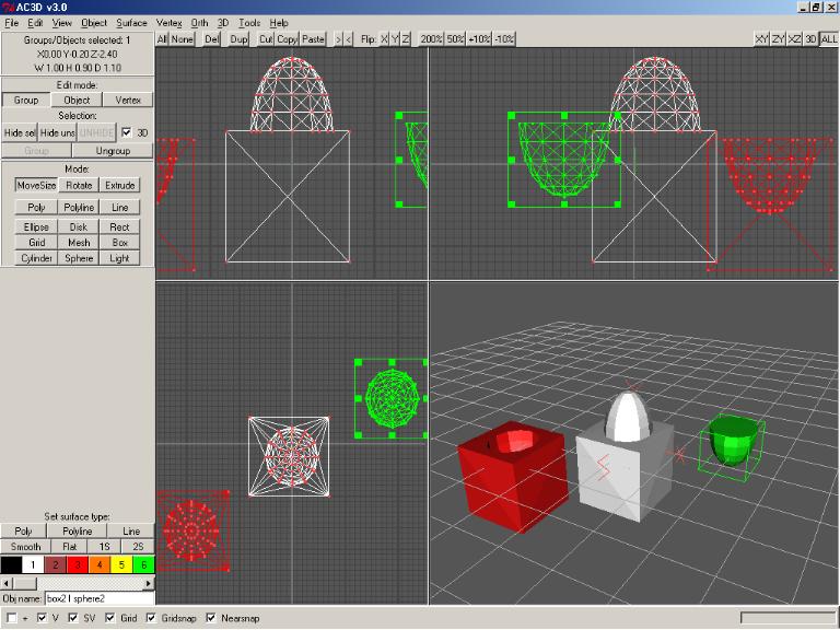
Any objects created can be used immediately within PHOENICS:
Parallel PHOENICS has been available for several years, both for multi-processor machines and for clusters of single-processor ones.
Many PHOENICS users have therefore been enabled to carry out simulations that would have been prohibitively time-consuming if run in sequential mode.
Parallel PHOENICS makes use of "domain-decomposition"; but, until now, it has been possible to split the domain of study only in the z-direction.
However, many large simulations do not have a grid that is significantly larger in one direction than the others; and indeed many large two-dimensional problems have been formulated so as to use the x- and y-directions only; for that is the most economical choice for sequential machines.
The ability to split the domain in all three directions is therefore very desirable, so as to increase the efficiency of the operation and to enable a larger number of processors to be used.
PHOENICS-3.5 now possesses this ability. The enhancement enables parallelisation to be applied to a much wider range of cases than before.
(Note: this feature is currently available only on LINUX and UNIX systems; Windows-based PCs will be added to the list shortly.)
It was particularly the last development which showed how non-uniform the internal handling of material properties had become, because of its history; and which therefore motivated its reorganization.
As a consequence of this reorganization, all properties are now handled in a uniform manner, in that they can be:
Although older methods of property-setting are still operational, it is the use of In-Form's (PROPERTY ....) statement which is recommended.
To assist users to understand, and benefit from, the new treatment, a "properties" document (TR 004) has been added to the hard-copy documentation.
The main development connected with the multi-fluid model of turbulence has been the provision of means of solving for "continuously-varying attributes".
Therefore, if the gases in a turbulent combustor are treated as a population of, say, 20 different fluids, distinguished by their fuel-air ratio, each is now allowed to possess its own non-discretised temperature, density and NOX concentration.
This new feature of PHOENICS-3.5 is being employed both for combustor simulations and for the gravity-influenced turbulence in stratified marine waters.
There have been two main developments in this area, namely:
Moreover the methods of specifying these properties have been brought into line with those used for the properties of fluids, as part of the reorganization mentioned in section 9.
CHAM is sponsoring PhD work on the subject at the University of Hertford.
The PARSOL feature of PHOENICS has many merits. In particular it enables flow around bodies of complex shape to be simulated without the use of body-fitted co-ordinate grids, as was already shown in the following picture which appeared in "What's New in PHOENICS 3.4":
However, its implementation in PHOENICS-3.4 had some limitations, of which one was acknowledged and (temporarily) accepted, while the other came to light only in the course of experience.
The acknowledged limitation was an insufficiently accurate representation of 'conjugate heat transfer', i.e. the circumstance in which heat transfer has to be computed between the fluid and the solid, and the thermal conductivity of the latter is not so great that its temperature can be taken as uniform.
By careful re-coding, coupled with painstaking testing, this limitation has been completely removed. as many newly-created examples in the Input Library have proved.
The following picture shows how the symmetry of the temperature distribution has been improved for conjugate heat transfer problem.
The old-PARSOL result is on the left; the new-PARSOL one is on the right.
The second limitation was a tendency to produce inaccurate results, even for flows without heat transfer, in certain circumstances, especially those in which body-defining facets lay very nearly in grid-defining planes.
This limitation has also been eliminated, by the adoption of a more robust algorithm for computing which facets cut which cell edges, and where.
It would be inappropriate to explain here the details of the new algorithm; but it is worth reporting that it has the further advantage of being much faster in execution than the previous one.
This is particularly important now that attention is being given to moving bodies, which require that the facet-cuts-cell behaviour must be recalculated at the start of each time step.
COFFUS
is the name of a special-purpose version of PHOENICS which simulates flow, heat transfer and combustion in large furnaces.It was created within the framework of the EC-supported MICA project; and it is now the focus of attention of another such project entitled Nice-Coal.
Several related developments are now available within PHOENICS-3.5, as described below;
The model is an extension of COFFUS approach significantly improving its physical basis and robustness in terms of radiation, coal-drying, char-oxidation and NOX production modelling.
The PHOENICS Input-File Library contains nearly three thousand cases; and more are being added every week. However, the more there are, the harder it becomes to find what one wants,
CHAM has therefore developed a library-search facility which enables all cases satisfying a selected set of criteria to be listed and then inspected and run.
The user selects one or more of features connected:
This facility is activated by way of the New PHOENICS Commander, which has replaced both the earlier Commander and the PHOENICS Manager.
Although much of the world uses Systeme Internationale (SI) units of measurement, the so-called Imperial system (lb, ft, hr, Btu) is still widely used, especially in North America.
For this reason, CHAM has attached a units-converter utility to PHOENICS.
On-line readers can sample it by clicking here.
Others can gain an idea of what it does from the following picture:
Under development, and to be completed by the end of September 2002, is an improved PHOTON which, while capable of doing all that the current PHOTON can do, will:
As soon as this is complete and delivered, an in-PHOTON post-processing capability will be developed, which will enable users to compute and plot arbitrary functions of the variables with which it has been supplied.
The moving-frame-of-reference concept (MOFOR) was mentioned above in connexion with both In-Form and PARSOL.
This will be a subject on which CHAM will be focussing in the coming months because of its importance both in mechanical industry (pumps, impellers, missiles and vehicles) and in human motion (running, dancing and swimming).
PHOENICS users who have interest in such matters are invited to communicate their experiences, their wishes and their advice to CHAM.
The conduction term in the Enthalpy Equation
In all versions of PHOENICS prior to 3.5, the conduction term in the enthalpy equation has been written as -(k/Cp).grad(h). This meant that it was not possible to perform meaningful conjugate heat transfer calculations with the enthalpy formulation.
In PHOENICS 3.5, the temperature-enthalpy relationship is internally defined as:
T = (h-h_base)/Cp
where h_base stands for the enthalpy of the material in question when T equals 0.0 on the temperature scale in question. The values of h_base are deduced from the TMP1/2 and CP1/2 settings.
The conduction term at any solid-fluid interface has been written in the form -k.grad((h-h_base)/Cp), which is equivalent to -k.grad(T).
The consequences of this change are that
The Specific Heat and Temperature, CP1/TMP1 and CP2/TMP2
In Version 3.4 and earlier, the constants for the CP1 formulae were transferred to Earth via TMP1A, TMP1B and TMP1C. These constants were also used for the TMP1 temperature-enthalpy relationship.
In Version 3.5 new variables CP1A, CP1B and CP1C have been introduced to eliminate this double use, with CP2A etc for phase 2. The TMP1A/B/C variables are now used exclusively for TMP1. The specific heat previously implied by the TMP1A/B/C settings for the various TMP1 formulae, is now explicitly set via CP1.
Users who are using any of the built-in CP1/2 formulae must edit their Q1 files to change TMP1A to CP1A and so on.
Users who are using any of the built-in TMP1 formulae must also ensure that the CP1 setting is consistent with the selected TMP1 formula.
Bearing in mind that the enthalpy-temperature relationship is defined as:
T = (h-h_base)/Cp
the changes required for the various TMP1 (or TMP2) formulae are:
TMP1 |
Old formula, T= | New formula, T= |
| GRND1 | TMP1A | TMP1A |
| GRND2 | TMP1A+TMP1B*H1 | TMP1A+H1/CP1 user should set CP1=1/TMP1B h_base=-TMP1A*CP1 |
| GRND3 | TMP1A + TMP1B * H1 + TMP1C * C3 | TMP1A + H1/CP1 + TMP1C * C3 user should set CP1=1/TMP1B h_base=-(TMP1A+TMP1C*C3)*CP1 |
| GRND4 | TMP1A * H + TMP1B * AMAX0(0.0, C1 + TMP1C) | H/CP1 + TMP1B * AMAX0(0.0, C1 + TMP1C) user should set CP1=1/TMP1A h_base=-(TMP1B*AMAX1(0.0,C1)+TMP1C)*CP1 |
| GRND5 | (TMP1A - 0.5 * (U1**2 + V1**2 + W1**2)) / TMP1B | (TMP1A - 0.5 * (U1**2 + V1**2 + W1**2)) /CP1 user should set CP1=TMP1B |
| GRND6 | (H1 - 0.5 * (U1**2 + V1**2 + W1**2)) / TMP1B | (H1 - 0.5 * (U1**2 + V1**2 + W1**2)) /CP1 user should set CP1=TMP1B h_base=0.5 * (U1**2 + V1**2 + W1**2) |
| GRND7 | (H1 - TMP2B * Mfuel)/ (TMP1A * Mfuel + TMP1B * Mprod + TMP1C * Moxid) | (H1 - TMP2B * Mfuel)/CP1 user should set CP1=GRND10 and CP1A= TMP1A; CP1B=TMP1B; CP1C= TMP1C h_base=TMP2B*Mfuel |
Note that the CP1 settings given in bold in the table are those required to reproduce exactly the old formulae. Any CP1 formula can in fact be used. The h_base definitions are given for information; they are set internally in GXTEMPR.FOR.
Users who have set TMP1=GRND must ensure that h_base is calculated in such a fashion that the T=(h-h_base)/Cp relationship is satisfied. The indices IH01 and IH02 should be used to set the values. For example, to recreate the TMP1=GRND2 (T = a + bH) option, in Q1 set:
TMP1=GRND; RG(1)=const; CP1=value
In Group 9, Section 10 of Ground, put
      L0T1=LOF(TEMP1)
      L0H1=L0F(H1)
      L0CP1=L0F(ISPH1)
      L0H_BASE=L0F(IH01)
      DO I=1,NXNY
        F(L0T1+I)=RG(1)+F(L0H1+I)/F(L0CP1+I)
        F(L0H_BASE+I)=-RG(1)*F(L0CP1+I)
      ENDDO
The Property Marker Variable PRPS
The STOREd variable PRPS has long been used to mark the property number for each cell. In earlier versions of PHOENICS, the individual property variables, RHO1, ENUL, CP1 and PRNDTL(TEM1), had to be set to GRND10 to make EARTH find the property values from the PROPS file.
In PHOENICS 3.4 and 3.5, the very existence of PRPS as a STOREd variable is enough to make EARTH check the PRPS value for each cell. In Version 3.4, for cells in which PRPS=FIINIT(PRPS), EARTH would take the properties from RHO1, ENUL, CP1 and PRNDTL(TEM1), not the PROPS file.
If the user selected a material for the domain, say 67 - Water, then edited the properties of the material to change the density to 1001, the Q1 file would contain RHO1=1001; FIINIT(PRPS)=67.
In Version 3.5, the properties are taken from RHO1, ENUL etc in cells where PRPS=-1.0. For the above example, the user should change FIINIT(PRPS) from 67. to -1., otherwise the default density for material 67 will be used.
In addition, users who find settings such as:
RHO1=GRND10; ENUL=GRND10; CP1=GRND10; PRNDTL(TEM1)=GRND10
FIINIT(PRPS)=n
in their Q1 files are advised to delete these settings and add the line:
SETPRPS(1,n)
at the end of Group 9.
Turbulence Model Constants
The turbulence model constants for all variants of the K-e model can be set from the Q1 file using the SPEDAT command. These take the form:
SPEDAT(SET,KECONST,const,R,value)
where 'const' can be AK, EWAL,CMU, CD, C1E, C2E, GCE3, GCT1, GCT2 or GCT3, and 'value' is the required value. These constants are also available on the Main Menu / Settings panel for Turbulence in the VR-Editor.