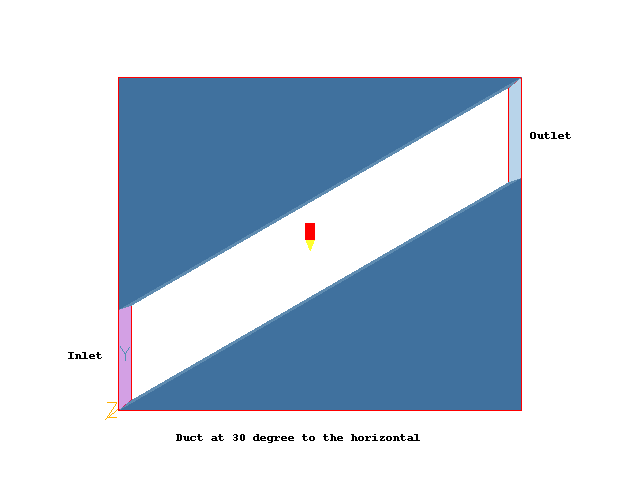
This workshop is designed to show the cut-cell technique called PARSOL. The geometry for the example is shown below.
The flow to be set up is a two-dimensional duct at 30° to the horizontal with frictionless walls.
The flow enters at 1.0 m/s, again at 30° to the horizontal. There should hence be no velocity profile across the duct, and no pressure drop along it.
The case will be first run without PARSOL activated and then with PARSOL activated and the results compared.
Start with an 'empty' case - click on 'File' then on 'Start New Case', then on 'Core', then click on 'OK'; to confirm the resetting.
Set the domain size, and activate solution of variables.
Click on 'Main Menu'.
Type 'The use of PARSOL' in the 'Title' box
Click on 'Geometry' and Switch Off 'Cut-cell method'.
Set the Domain size to 8.0 in the x-direction and 6.62 in the y-direction.
Click on 'OK' to close the Grid mesh settings dialog.
Click on 'Models' and set 'Solution for velocities and pressure' to 'ON'.
Select 'LAMINAR' for the turbulence models option.
Click on 'Top menu' and 'OK'.
Rotate the view to see the working plane (the X-Y plane).
Click 'Reset' on the Movement control panel, then 'Fit to window' and 'OK' to re-scale the view to fit the geometry.
Press the 'View down/move down' button to rotate the domain 90º so it can be viewed in the xy-plane rather than the default xz-plane. Alternatively, you may also click on 'Mouse' button and use the Mouse to rotate the view.
Click on 'Reset' then 'Nearest head-on' to align the view exactly with the Z axis.
Create the objects making up the scene
Click on the 'Object Management' button (O on the toolbar or
on the hand set). This will display a (currently empty apart from the domain) list of objects.
Create the first (upper) angled blockage
In the Object management dialog, click on 'Object', 'New', 'New Object', 'Blockage'.
Set the name to WEDGE1.
Click on the 'Size' button and enter:
XSize: 8.0
The slope is 30º, so the height of the lower wedge is 8*tan(30) = 4.62
YSize: 4.62
ZSize: tick 'To end'
Click on the 'Place' button and enter:
XPos: 0.0
YPos: tick 'At end'
ZPos: 0.0
Click on the 'Shape' button and select 'Geometry' from: PUBLIC/SHAPES/WEDGE and click on 'Open'
On 'Options' click 'Rotation options' and click the up arrow by 'Rotate object face' until the wedge is in the right position. This will be for position 6. Click OK.
Click on 'General' and 'Attributes'. Change the material to '199 Solid allowing fluid slip..'.
Click on 'OK'; and 'OK';.
Create the second (lower) angled blockage by duplication.
Click on 'Duplicate object' button and then click 'OK' to confirm the duplication.
Double-click the new object in the Object Management Dialog to open its dialog. Change the name to WEDGE2
Un-tick 'At end' for Y, and change the Y position to 0.0.
On 'Options' click 'Rotation options' and click the up arrow by 'Rotate object face' until the wedge is in the right position. This will be for position 18. Click OK and OK.
Create the fluid inlet
Click on 'Settings', 'New', 'New Object', 'Inlet', and select the X plane for the inlet to lie in.
Set the name to IN.
Click on 'Size' and enter:
XSize: 0.0
YSize: 2.0
ZSize: 'To end'
Click on 'Place' and enter:
XPos: 0.0
YPos: 0.0
ZPos: 0.0
Click on 'General'.
Click on Attributes and set:
X Direction velocity to 0.866 m/s (this is 1*cos(30))
Y Direction velocity to 0.5 m/s (this is 1*sin(30))
Z Direction velocity to 0.0 m/s
Click on 'OK'; and on 'OK';.
Create the fluid outlet
Click on 'Settings', 'New', 'New Object', 'Outlet', and select the X plane for the outlet to lie in.
Set the name to OUT.
Click on 'Size' and enter:
XSize: 0.0
YSize: 2.0
ZSize: 'To end'
Click on 'Place' and enter:
XPos: 'At end'
YPos: 'At end'
ZPos: 0.0
Click on 'OK';
Setting the Probe Location
Click on the probe icon
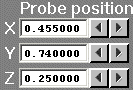
on the toolbar or double-click the probe itself, and move the probe to X=4.0, Y=3.31, Z=0.5.
Set remaining Solution Control parameters
Click on 'Main Menu'.
Under 'Numerics' and set 'Total number of iterations' to 350,
Click on 'Top menu' and on 'OK';.
In the PHOENICS-VR environment, click on 'Run', 'Solver', and click on 'OK' to confirm running Earth.
In the PHOENICS-VR environment, click on 'Run', 'Post-processor', then GUI Post processor (VR Viewer) Viewer)'.
Click 'OK' on the file names dialog to accept the default files.
To view:
To select the plotting variable:
To change the direction of the plotting plane, set the slice direction to X, Y or Z ![]()
To change the position of the plotting plane, move the probe using the probe position buttons
 .
.
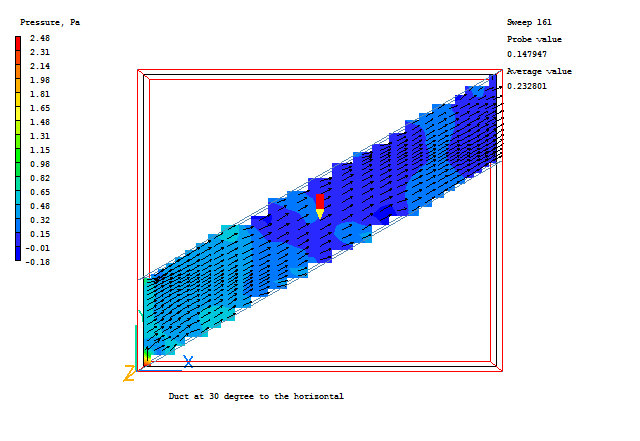
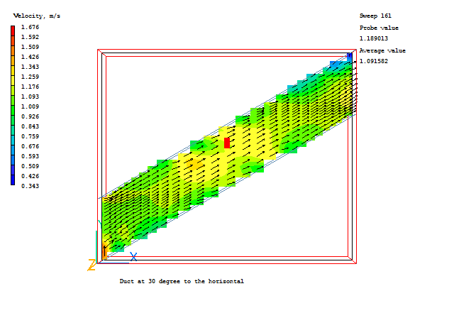
In particular, note the non-uniform velocity vectors, and the pressure drop from inlet to outlet.
In the PHOENICS-VR environment, click on 'File', 'Save as a case', make a new folder called 'PARSOL' (e.g.) and save as 'CASE1' (e.g.).
Click on 'Run - Pre processor - GUI Pre processor (VR-Editor)' to return to the Editor.
Activate PARSOL.
Click on 'Main Menu'.
Click on 'Geometry' and set Cut-cell method to PARSOL.
Exit from the Main Menu.
In the PHOENICS-VR environment, click on 'Run', 'Solver', and click on 'OK' to confirm running Earth.
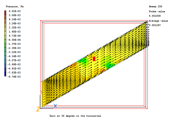
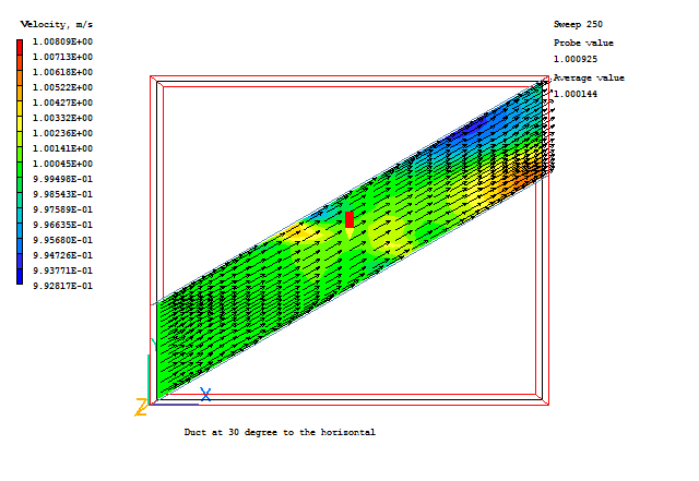
View the results using the VR Viewer. Note the minimal velocity variation, and the small pressure drop from inlet to outlet.
Compare the results for the velocities and pressure drops for the two cases.
In the PHOENICS-VR environment, click on 'Save as a case', make a new folder called 'PARSOL' (e.g.) and save as 'CASE2' (e.g.).