This workshop shows the user how to set up a simple case which simulates the 2d turbulent flow of solid particles over a backward facing step.
Air, laden with solid particles, enters a 2d plane channel with a velocity of 13 m/s. The total channel width is 0.1143m and the length of the channel is 0.762m. The step is 0.1524m long by 0.0381m high. Turbulence is represented by means of the standard k-e model with equilibrium wall functions.
The density and diameter of the particles is 1500 kg/m3 and 10 microns, respectively. 60% of the particles enter with the air, and the remaining 40% are released near the base of the channel about 0.05m downstream of the step. The mass loading of the particles is about 1% of the air flow.
The particulate phase is represented by 5 tracks of equal mass loading. The initial position and velocity vector of each track are defined below:
| Track 1 | X = (0, 0.09) | U = (11.25, -6.5) |
| Track 2 | X = (0, 0.07) | U = (11.25, -6.5) |
| Track 3 | X = (0, 0.05) | U = ( 5.63, -0.4) |
| Track 4 | X = (0.2, 0.05) | U = ( 1.80, -0.6) |
| Track 5 | X = (0.2, 0.01) | U = ( 8.50, -0.3) |
From the system level:
To enter the PHOENICS-VR environment, click on the PHOENICS icon on the desktop, or click on Start, programs, PHOENICS, PHOENICS.
In PHOENICS-VR environment:
The first task is to load the backward-facing-step case from the PHOENICS library so as to provide a working fluid-flow Q1 file for use with GENTRA.
Click on 'File', 'Load from Libraries', enter 300 in the Case Number data entry box, and click 'OK'.
The case now needs to be modified so as to increase the number of iterations for complete convergence, and to activate the Graphical Display Monitor when running EARTH. Therefore, click on 'Menu' then on 'Numerics' Change the total number of iterations to 150. Click on 'Output', and toggle Monitor display mode from 'ASCII' to 'Graphics'. Click 'Top Men' then 'OK' to leave the main menu.
As a benchmark, the case can now be run without particles. Run the EARTH solver by clicking on 'Run', 'Earth' and 'OK'. Save these results by clicking on 'File', 'Save as a case'. Enter the case name GENTRA-0.
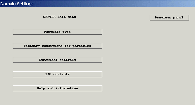
Loading the GENTRA Menu:
Click on 'Menu', then on 'Models'. Toggle Lagrangian Particle Tracker (GENTRA) to 'ON', then click on 'Settings'. The following menu panel will appear:
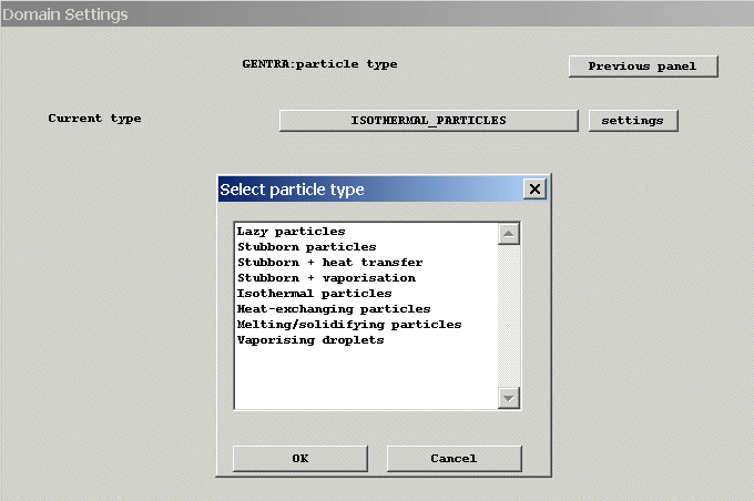
Select the particle type:
Click on 'Particle Type' so as to display the Particle type menu. The default particle type is 'Isothermal Particles'. This type is appropriate when only momentum transfer is to be considered between the continuous and disperse phases.
Other particles types can be selected by clicking on 'Isothermal_particles'. For this example we do not need to change the particle type.
Set the physics of the particle:
Click 'Settings' for the Menu option 'Current type'. As can be seen below, this Menu allows the user to specify the drag coefficient, introduce gravitational or buoyancy forces on the particle, and also activate the stochastic turbulence model for particle tracking.
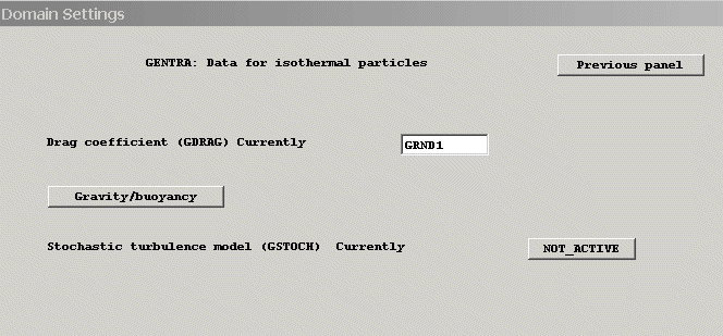
The built-in drag law GRND1 for solid spheres will suffice. Then return to the previous Menu panel by clicking on 'Previous panel' twice.
Setting the boundary conditions for the particles:
Click 'Boundary conditions for particles'. The following panel will appear:
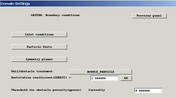
Inlet conditions
Click on 'Inlet conditions'.
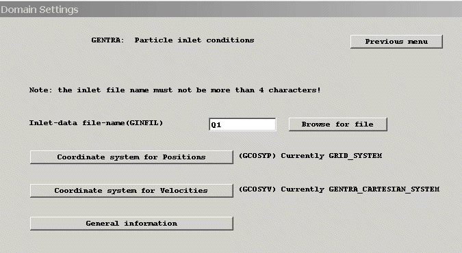
The particle inlet conditions must be specified by means of a inlet-data file or directly in the Q1 file after the GENTRA Menu session.
For this example, the inlet data for the particles are to be supplied in the Q1 file, which is the default setting. Click on 'Previous panel'
Particle Exits
Particle exit conditions are set individually for all Inlet, Outlet and Fan objects. By default, particles are allowed to leave through all Inlet, Outlet and Fan objects. The entry here provides help information.
Symmetry Planes
These are set as Objects. The entry here provides help information. This case does not require any Symmetry planes.
Wall/Obstacle treatment
The task here is to specify how the particles interact with walls and obstacles, e.g. bouncing, sticking, removal.
The default is for the particles to bounce. Enter a restitution coefficient of 0.75.
Click on 'Previous panel' to return to the GENTRA Main Menu.
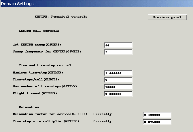
Setting the Numerical Controls:
Click on the 'Numerical controls' to select the 'Numerical controls' Menu.
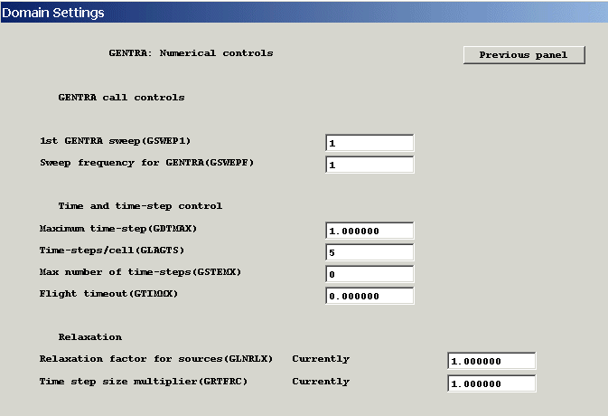
Enter '20' for the 1st GENTRA sweep.
Enter '10000' as the maximum number of time steps.
Enter '3.0' as the flight time out for a particle.
Click on 'Previous panel' to return to the 'GENTRA Main Menu'.
Setting the Input/Output Controls:
From the 'GENTRA Main Menu', click on 'I/O Controls '. The following Menu panel will appear on the VDU.
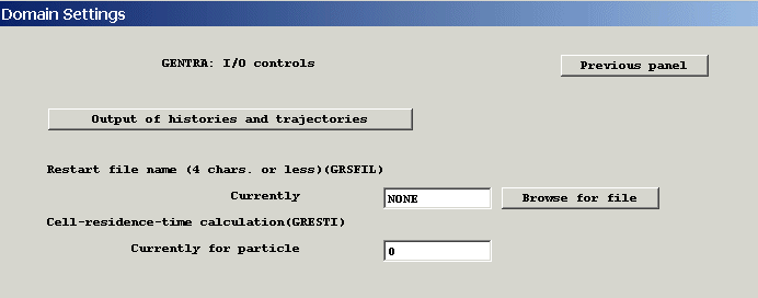
Output of histories and trajectories:
Click 'Output of histories and trajectories' to display the following Menu panel.
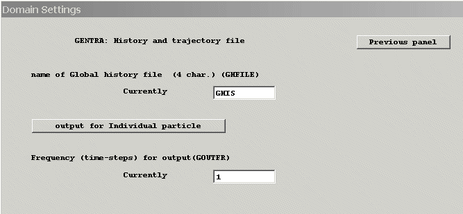
Since we require individual history and trajectory files, click on 'Output for Individual particle', and then the following menu panel appears.
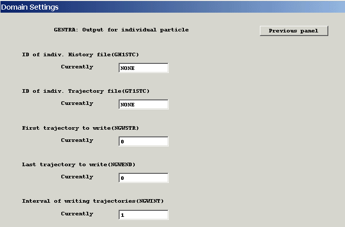
Enter 'H' as the first character for the name of the individual history file.
Enter 'T' as the first character for the name of the individual trajectory file.
Enter '1' as the first track for which an individual history-trajectory
file is required.Enter '5' as the last track for which an individual history-trajectory
file is required.Click on 'Previous panel' twice to return to the 'I/O controls Menu'.
Click 'Previous panel' twice more to return to the Main Menu.
Click 'Top Menu' and 'OK' to leave the Main menu and return to the VR-Editor.
3) Defining the Inlet Conditions for the Particles.
The task is now to specify the particle inlet conditions in the Q1 file.
For more detailed information than is given here, the user is referred to the instructions given in Section 2.7.1 of the GENTRA User Guide TR211.
Click on 'File', then on 'Open file for editing', and then on 'Q1'. Click on 'Yes' when prompted to save files.
Now insert the lines of inlet data between the two special marks provided by the GENTRA Menu Session, i.e. <GENTRA-INLET-DATA> and <END-GENTRA-INLET>.
Please note that the inlet-data lines must not start in the 1st or 2nd column of the Q1 file, and the length of the data should not exceed column 68 in the Q1 file.
The final result is shown in the following extract from the Q1 file:
        *-------------------------------------------------------
        * GENTRA GROUP 2: Boundary conditions for particles
        *-------------------------------------------------------
        * Inlet-data file-name
      GINFIL  ='Q1'
       <GENTRA-INLET-DATA>
         * X         Y       U     V     DIA    RHO   MASSFLO
         0.0E+00  9.0E-02   11.25 -6.5  1.E-05  1500.  2.00E-03
         0.0E+00  7.0E-02   11.25 -6.5  1.E-05  1500.  2.00E-03
         0.0E+00  5.0E-02   5.63  -0.4  1.E-05  1500.  2.00E-03
         2.0E-01  0.5E-02   1.80  -0.6  1.E-05  1500.  2.00E-03
         2.0E-01  1.0E-02   8.54  -0.3  1.E-05  1500.  2.00E-03
       <END-GENTRA-INLET>
It may be convenient to use 'Copy' and 'Paste' to insert the above settings.
In addition, increase LSWEEP from 150 to 200 in Group 15 in the Q1 file, as more sweeps will be needed for convergence of the GENTRA run.
Now save the modified Q1 by clicking on ‘File’, 'Exit' and 'Yes'. Allow VR to re-load themodified Q1.
4) Running the GENTRA CFD Solver.
Run EARTH by clicking on'Run', 'Solver'(Earth) and 'OK'.
5) The GENTRA Output Files.
In addition to the usual RESULT and PHI file, the EARTH run will produce the following output files:
h00001 h00002 h00003 h00004 h00005 t00001 t00002 t00003 t00004 t00005 genuse The files h0001, h0002, etc are the history files, one for each track.
The files t0001, t0002, etc are the trajectory files, one for each track.
The file genuse is used to plot the trajectories of all tracks simultaneously in PHOTON.
The history files provide a tabular output of the particle history of each requested track, and these files may be read into AUTOPLOT to produce x-y line plots, such as for example, plots of the particle axial velocity against time.
At each requested Lagrangian time step, the following data are written to each history file:
PR.No. TIME XPAR YPAR ZPAR UCPAR VCPAR WCPAR DIAM TPAR TGAS SFRC where
PR.No is an integer identifying the number of the track, e.g. 1 for track 1.
TIME is the time in s.
XPAR, YPAR and ZPAR are the Cartesian coordinates of the particle position vector in m.
UCPAR, VCPAR and WCPAR are the Cartesian components of the particle velocity vector in m/s.
DIAM is the particle diameter in m.
TPAR is the particle temperature in K.
TGAS is surrounding fluid temperature in K.
SFRC is the solid mass fraction.
TPAR, TGAS and SFRC are not relevant in the present example.
6) Using VR-Viewer & AUTOPLOT to display the Results.
VR-Viewer
Click on 'Run', 'Post processor',then GUI Post processor(VR Viewer)'.
When the file dialog appears, click 'OK' to use the default files.
The fluid velocity vectors can be displayed by clicking on the Vector toggle
on the handset. To colour the vectors by Velocity, click the 'Select velocity button'
.
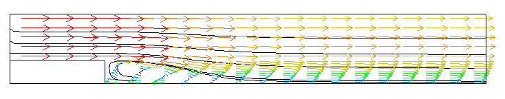
The particle trajectories are displayed by using the macro file written by EARTH. Click on 'Macro' and then enter 'GHIS' as the name of the macro file to run. Click 'OK' to close the dialog and plot the particle paths as shown below.
.
Next, Contour plots of the Cartesian components of the interphase momentum force vector can be made, as follows:
Click on the 'Contour toggle'
to turn on the contour display. Click on the 'Select variable'
button and select 'MOMX' from the list for the forces in the X direction, and then click on 'OK'.
Repeat this procedure so as to plot contours of MOMY, i.e. the forces in the Y direction.
AUTOPLOT
In the PHOENICS-Commander environment, click on 'Run, Post processor,X-Y Graph plotter (AUTOPLOT)' and after AUTOPLOT has loaded enter 'FILE' <CR>, and then the following commands:
H00001 2 <CR>
H00002 <CR>
so as to load the history files for tracks 1 and 2.
Temporal plots of the axial component of the particle velocity vectors of tracks 1 and 2 can
now be displayed by entering the commands:
D 1 TIME UCPAR <CR> (creates data element 1 from data file 1, i.e. H00001) D 2 TIME UCPAR <CR> (creates data element 2 from data file 2, i.e. H00002) COL3 1;COL9 2 <CR> (makes an x-y plot of UCPAR against TIME for tracks 1 and 2) Enter the command END <CR> to exit AUTOPLOT and return to the PHOENICS Commander.
7) Further Suggestions.
You may now like to create a more demanding problem by using the GENTRA Menu to activate the Stochastic turbulence model.
First, save the current model by clicking on 'File', 'Save as a case'. Enter GENTRA-1 as the case name.
Stochastic tracking
The stochastic model allows for the turbulent dispersion of particles as they cross eddies during their trajectories.
Click on 'Run - Pre processor - GUI Pre processor (VR-Editor)' to return to the Editor.
Click on 'Menu', 'Models' and then on 'Settings' to enter the GENTRA Main Menu.
From the 'GENTRA Main Menu', click on 'Particle Type' so as to display the Particle-type Menu.
Next, click 'settings' for the Menu option 'Data for Isothermal Particles'.
Finally, activate the 'Stochastic turbulence model'.
Click 'Previous panel' three times to return to the Main Menu, then 'Top Menu', 'OK' to exit the main menu'.
Run EARTH by clicking on'Run', 'Solver'(Earth), and you will find that convergence is more problematic with the stochastic model.
Convergence control
You can try to improve the convergence behaviour by using more sweeps (say 500), more inertial relaxation on the fluid momentum equations (say 1.E-3 s), and using linear relaxation on KE and EP (say 0.3). These changes to the fluid-phase numerical parameters should be made from the 'Numerics', 'Relaxation control' panel of the Main Menu.
Other things to try are the numerical controls for GENTRA particle tracking algorithm.
From the 'GENTRA Main Menu', click on 'Numerical controls' so as to display the Numerical controls Menu.
The foregoing particle-phase settings together are suggested to secure improved convergence behaviour.
Exit the Menu.
Run EARTH by clicking on 'Run' and then 'Earth'.