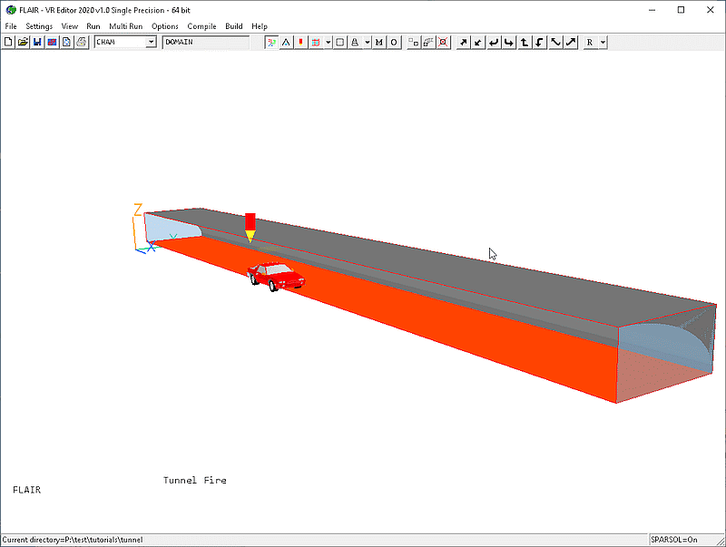
This example the flow resulting from a car fire in a short tunnel. The heat source is put in as a piece-wise linear source for a FIRE object.
The geometry of the case is shown in Figure 1 below. There are openings (outlets) at either end. The external temperature is 25°C.
Only half the tunnel width is represented, so there is a symmetry plane at y=0. The car geometry is only representative. The tunnel is inclined at 2°.

Figure 1. The geometry of the In-Form example
The heat source will be set to:
| Time s | Heat Source W |
| 0 | 0 |
| 300 | 3000000 |
| 720 | 3000000 |
| 915 | 5000 |
| 1200 | 5000 |
A complete step-by-step guide, showing how to set the case from the default mode of operation, is provided below.
Start FLAIR with the default room
The FLAIR VR-Environment screen should appear, which shows the default room with the dimensions 10mx10mx3m.
Set the domain size and grid numbers:
Click on 'Menu' (Main Menu) on the VRE-Editor panel (or the M icon on the tool bar); and then on 'Geometry'.
Set the x-domain size to 50.0.
Set the y-domain size to 5.0.
Set the z-domain size to 2.5.
Turn the 'Auto' settings for X, Y and Z to 'Manual', and set 'number of cells' to 40 in the x-direction, 5 in the y-direction and 20 in the z-direction. This is too coarse for an accurate solution, but will allow the tutorial to run relatively quickly.
Click on Time dependence 'Steady' to change to 'Transient'. Click on 'Time step settings'. Set the last time step number to 65, and the Time at end of last step to 1200s. Click on 'Split regions', and create a new region boundary at 10s. Set 10 steps for time region 1, and 55 for time region 2. This will make the first 10 steps 1s each, and the remainder to 21.6s. Click 'OK' to close the time step dialog. The change in time step size is probably too large, but illustrates the method of setting different step sizes.
Click on 'OK' to close the Grid mesh settings dialog.
The domain no longer fits the screen. To resize the view so that it does fit, click on the pull-down next to the 'R' icon on the toolbar then 'Fit to Window' and then repeat for 'View -Y'.
Models settings
On the Top Panel, enter 'Tunnel Fire' as the Title.
Click on 'Models'.
Leave 'Solution for velocities and pressure' at ON. Leave Energy at TEMPERATURE.
Click on Chen-Kim KE (Turbulence models) and choose Constant-effective. This is a very simple turbulence model used to make the tutorial run faster.
Switch solution of Smoke mass fraction ON, then click Settings. The default smoke settings are suitable for a car fire, so we do not need to change anything. Switch the 'Sight length for light reflecting objects' to ON. Click 'Previous panel'.
Physical properties
Click on 'Properties'. Leave the domain material as '2 Air using Ideal Gas Law STP'.
Note that the ambient pressure and temperature are 1atm and 20°C respectively. Set the Ambient temperature to 25°C.
'Initialise from ambient' is ON, so the initial values of pressure and temperature throughout the domain will be set to these values.
Initial Values
Click on 'Initialisation'. You will see that the initial values for P1 (pressure) and TEM1 (temperature) are both set to AMBIENT.
Set Whole-domain sources
Click on 'Sources'. Gravitational forces are ON by default, using the Density-difference form .
The tunnel is to be tilted at 2° with Z pointing up. The Z component of gravity is therefore -9.81*cos(2). To tilt at 2° set the X component to -9.81*sin(2) which is -0.34. Set the components of the gravity vector to (-0.34,0.0, -9.804) in (x,y,z).
The reference density should be set to that at which the flow is neutrally buoyant - in this case 25°C.
On the Properties panel, 'Set buoyancy from ambient' was ON so the reference density has been set automatically from the ambient pressure and temperature. The value should be the density of air at 25°C, which is 101325/(287*(25+273)) = 1.1847 kg/m3.
Enter numerical settings
Click on 'Numerics'.
Set 'Total of number of iterations' to 50.
Set output controls
Click on 'Output', then on 'Settings' next to 'Write flow field'. Set 'Intermediate field dumps' to ON. Set the step frequency for dumping to 1, and the start letter for PHI (CSG1) to a. The Earth solver will write files called a1, a2, a3 and so on.
Click on 'Top menu' and then on 'OK' to exit from 'Menu'.
Create Objects and specify boundary conditions
Click on the 'Object Management' button (O on the toolbar or ![]() on the hand set). This will display a (currently empty
apart from the domain) list of objects.
on the hand set). This will display a (currently empty
apart from the domain) list of objects.
Create the openings
In the Object management dialog, click on 'Object', 'New' and 'New Object', 'Opening' and select the X plane.
Change name to UP.
Set Position and Size of the object as:
Xpos: At end, Xsize: 0.0
Ypos: 0.0, Ysize: To end
Zpos: 0.0, Zsize: To end
Click on 'Attributes'
You will see that the External temperature is set to 'User-set' and the value is set to 'Ambient'. The external velocities are set to 0.0.
Click 'OK' to exit from the Object Dialogue Box.
In the Object management dialog, click on 'Object', 'New' and 'New Object','Opening' and select the X plane.
Change name to DOWN.
Set Position and Size of the object as:
Xpos: 0.0, Xsize: 0.0
Ypos: 0.0, Ysize: To end
Zpos: 0.0, Zsize: To end
The default attributes will be as for the UP object, so do not need changing.
Click 'OK' to exit from the Object Dialogue Box.
Create the Roof Object
In the Object management dialog, click on 'Object', 'New' and 'New Object', 'Blockage'.
Change name to ROOF.
Set Position and Size of the object as:
Xpos: 0.0, Xsize: To end
Ypos: 0.0, Ysize: To end
Zpos: 0.0, Zsize: To end
On the 'Shape' tab, in 'Geometry', select public\Basic_Shapes\corner. The new shape is not aligned correctly. Click on 'Options' then 'Rotation options'. The 'Rotate object face' entry sets the orientation of the shape within its bounding box. There are 24 possible orientations. Keep changing the orientation number until you find the one which makes the shape lie correctly (it is number 10). An alternative way to do the same job is to repeatedly click on the 'Rotate object up/down' buttons
on the handset (if it is visible).
Click on 'OK' to exit the Rotation Options menu,
Click 'OK' to exit from the Object Dialogue Box.
Create the Ground plane
In the Object management dialog, click on 'Object', 'New' and 'New Object', 'Plate' and select the Z plane.
Change name to GROUND
Set POSITION and SIZE of object as:
Xpos: 0.0, Xsize: To end
Ypos: 0.0, Ysize: To end
Zpos: 0.0, Zsize: 0.0
Click on 'Attributes'. Set the Energy source to 'Surface Temperature'. Set the surface temperature to 25.
Create the Fire object
In the Object management dialog, click on 'Object', 'New' and 'New Object', 'Fire'.
Change name to FIRE1.
Click on 'Geometry' on the 'Shape' tab. Open the folder 'public\Equipmt', and select 'car4' and click 'OK'.
Set the Size as:
Xsize: 4.7
Ysize: 2.0
Zsize: 1.3
We are only modelling half the tunnel, so the car can be placed so that one half is outside the domain.
Click on 'Options' and un-tick 'Object constrained by domain'. Set the Position as:
Xpos: 23.0
Ypos: -1.0
Zpos: 0.0
Click on 'Attributes' on the 'General' tab
Set heat source to 'Piece-wise linear in time', then click 'Edit Heat source table'. Enter the following values:
Time s Heat Source W 0 0 300 1500000 720 1500000 915 2500 1200 2500 Note that as we are only modelling half the car, we should put in half the heat source.
Set the Mass Source and Scalar Source both to 'Heat related'.
Click 'OK' to exit from the Object Dialogue Box.
Create a Point-History Object
Point_history objects can be used to 'instrument' the solution. At each Point_history object the time-histories of pressure, velocity and temperature will be written to the RESULT file. In the Object management dialog, click on 'Object', 'New' and New Object', 'Point_history'.
Change name to MONIT.
Set POSITION and SIZE of object as:
Xpos: 22.5 Xsize: 0.5
Ypos: 0.0 Ysize: 0.5
Zpos: 2.0 Zsize: 0.1
The actual size entered does not really matter, as it will be reset to fill the cell nearest the specified position.
Click 'Attributes', 'Select variable for plotting' and add the SMOK and SLEN variables to the list. Click 'OK'.
All settings are now complete. The user should move the probe (small red pencil sign)
to the position shown in Figure 1 (roughly x=22, y=0, z=2.2) before running the Solver,
EARTH. Click on the probe icon ![]() on the toolbar or double-click the probe itself to move it.
on the toolbar or double-click the probe itself to move it.
In the PHOENICS-VR environment, click on 'Run', 'Solver' then 'Local solver(Earth)', and click on 'OK'; to confirm running Earth.
In the PHOENICS-VR environment, click on 'Run', 'Post processor',then GUI Post processor (VR Viewer) Viewer)'. Click 'NO' next to Use intermediate step files and turn to 'YES'. Click 'OK' to accept starting with the file for step 1.
To view:
To move on to the next time step, click or press F8. To go back one step, click or
press F7. To jump to any other saved step, click or press F6. To cycle through all saved
files, click the 'Animation' ![]() button.
button.
Figure 2 shows the velocity vectors and temperature contours on the Y=0 plane after 312s.
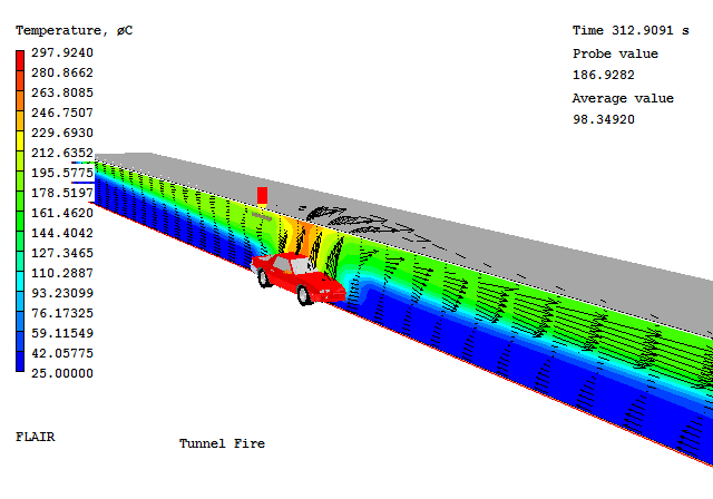
Figure 2. Velocity vectors and temperature contours at 312s
Figures 3,4 & 5 show iso-surfaces of 125C at 118s, 312s and 853s
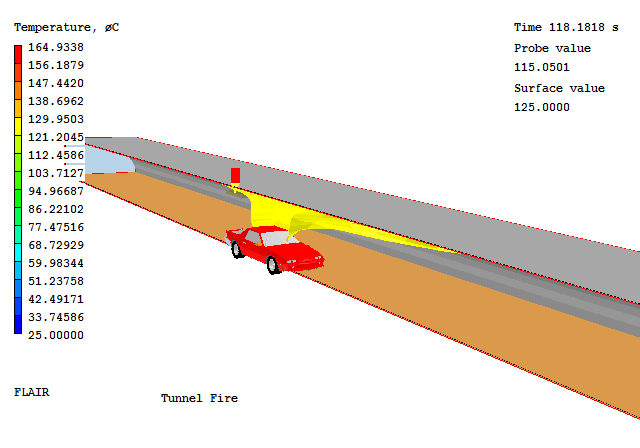
Figure 3. iso-surface of Temperature = 250°C after 118s
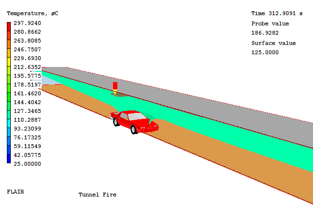
Figure 4. iso-surface of Temperature = 250°C after 312s
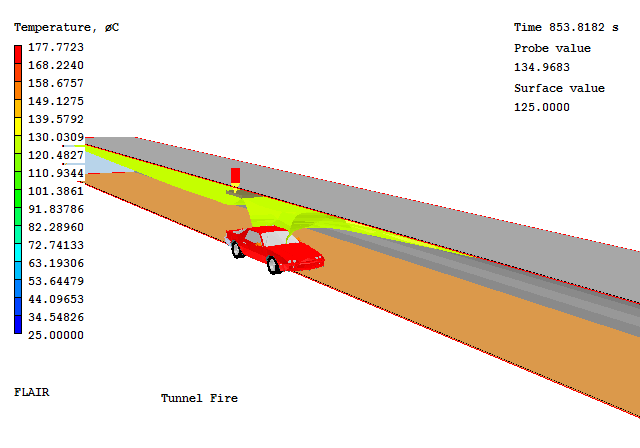
Figure 5. iso-surface of Temperature = 250°C after 853s
Figure 6 shows the time-history of temperature at the Point_history object MONIT. To get this image, select the MONIT object, right-click and select 'Show results'. Select TEM1 from the list of variables.
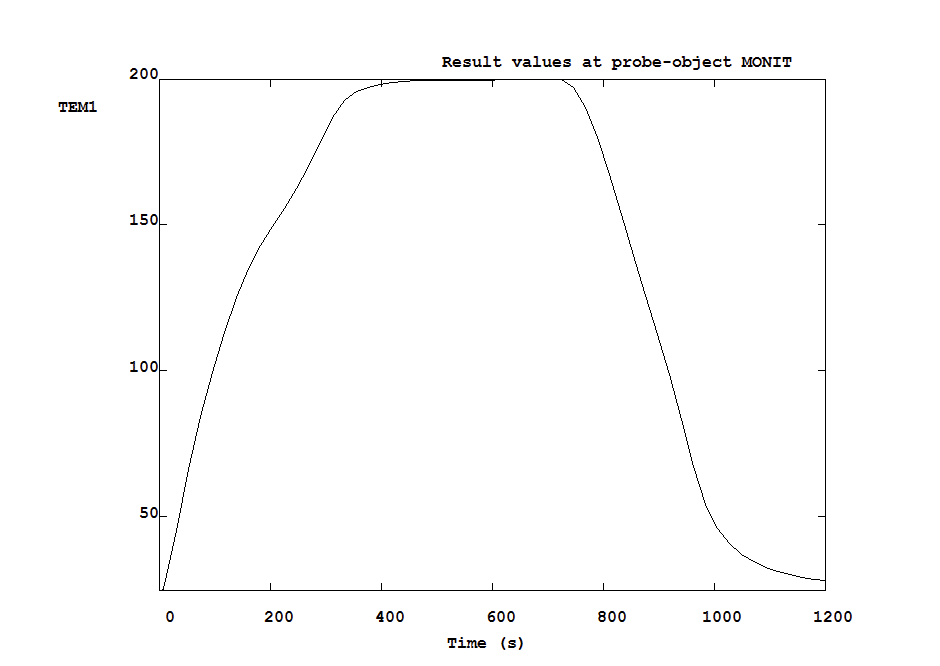
Figure 6. Time history of Temperature at MONIT
In the PHOENICS-VR environment, click on 'Save as a case', make a new folder called 'Flair', select the new folder, and save as 'FIRE'.