FLAIR Tutorial 6: A fan mounted at the boundary of a cabinet
This case shows how to activate the "Fan Operating Point" option for a single
fan mounted at the boundary of a cabinet as shown below.
Setting up the model
Start FLAIR with the default room
- Click FLAIR icon (a desktop shortcut created by the FLAIR installation program); or
- Start the VR-Editor by clicking on 'Start', 'Programs', 'FLAIR', then 'FLAIR-VR'.
- Click on the 'File' button and then select 'Start new case', followed by 'FLAIR' and
'OK'.
The FLAIR VR-Environment screen should appear, which shows the default domain with the
dimensions 10mx10mx3m.
Set the cabinet size
Change the X size to 0.5m
Change the Y size to 0.5m
Change the Z size to 0.7m
- Click on "Reset" button,
 on the movement panel, then click "Fit to window" and
then the 'OK' button.
on the movement panel, then click "Fit to window" and
then the 'OK' button.
Adding objects to the cabinet
a. add the top vent
- Click on the 'Object' menu and select 'New' (New Object), 'Opening' then select 'Z plane' on the 'Object management'
dialog box to bring up the 'Object specification' dialog box
- Change name to 'VENT'.
- Click on the 'Size' button and set 'Size' of the object as:
X: 0.3 m
Y: 0.2 m
Z:0.0 m
- Click on the 'Place' button and set 'Position' of the object as:
X: 0.1 m
Y: 0.15 m
Z: tick 'at end'
b. add the fan object:
- Click on the 'Object' menu and select 'New' (New Object), 'Fan' and select 'Y plane' on the 'Object management'
dialog box to bring up the 'Object specification' dialog box
- Change name to 'FAN'.
- Click on the 'Size' button and set 'Size' of the object as:
X:0.2 m
Y:0.0 m
Z:0.3 m
- Click on the 'Place' button and set 'Position' of the object as:
X: 0.15 m
Y: 0.0 m
Z: 0.2 m
- Click on 'General' button then 'Attributes' button to bring up the attributes dialog
- Change 'Include in matching' to YES.
- Click 'Fan Type' and select FAN1 from the list. We will check FAN1 data later.
- Set 'Fan Axis Direction' to 'POSITIVE'.
- Click on 'OK' to return to the object specification dialog box.
c. add the first chip
- Click on the 'Object' menu and select 'New' (New Object), 'Blockage' on the 'Object management'
dialog box to bring up the 'Object specification' dialog box
- Change name to 'CHIP1'.
- Click on the 'Size' button and set 'Size' of the object as:
X:0.05 m
Y:0.07 m
Z:0.02 m
- Click on the 'Place' button and set 'Position' of the object as:
X: 0.15 m
Y: 0.15 m
Z: 0.35 m
- Click on 'General' button
- Click on 'Attributes' button to bring up the attributes dialog
- Change 'Types' to 'Solids'
- Change the Material to 100 ALUMINIUM at 27 deg C.
- Change the Energy source to 'Fixed Heat Flux' and 'Total Heat Flux'
- Change the Value to 0.5 W
- Click on 'OK' to return to the 'Object specification' dialog box
- Click on 'OK' to close the Object specification' dialog box
d. add the second chip by duplicating CHIP1
- Highlight the CHIP1 object on the 'Object management' dialog box
- Click on the 'Duplicate object or group' button and click OK.
- Double click on the newly duplicated object to bring up the 'Object specification'
dialog box
- Change the name to CHIP2
- Click on the 'Place' button and set 'Position' of the object as:
X: 0.3 m
Y: 0.15 m
Z: 0.35 m
- Click on 'General' button
- Click on 'Attributes' and change the total heat flux value to 0.7
- Click on 'OK' to return to the attributes dialog
- Click on 'OK' to close the Object specification dialog
e. add the PCB
- Click on the 'Object' menu and select 'New' (New Object), 'Blockage' on the 'Object management'
dialog box to bring up the 'Object specification' dialog box
- Change name to 'PCB'.
- Click on the 'Size' button and set 'Size' of the object as:
X:0.3 m
Y:0.3 m
Z:0.01 m
- Click on the 'Place' button and set 'Position' of the object as:
X: 0.1 m
Y: 0.1 m
Z: 0.34 m
- Click on 'General' and then the 'Attributes' button to bring up the attributes dialog
- Change 'Types' to 'Solids'
- Change the Material to '101 BAKELITE at 20 deg C'.
- Click 'OK' to return to Object Management Box
Now we have 5 objects listed in the 'Object management' dialog box as shown below
To activate the physical models
a. The Main Menu panel
- Click on the 'Main Menu' button. The top page of the main menu will appear on the
screen.
- Click on the 'Title' dialogue box. Type in 'A cabinet with a fan'.
To activate 'K-E' turbulence model
- Click on 'Models' to obtain the Model menu page.
FLAIR always solves pressure and velocities. The temperature is also solved as the
default setting.
The 'Models' page of the Main Menu.
to activate 'Fan operating point' option
- Change 'Fan operating point' option from 'OFF' to 'ON' with default settings
- Click on 'Settings' for 'Fan operating point', then click 'Edit' next to
'Fan data file' on the next dialog. The
fandata file will be opened in the default file editor. Scroll down to FAN1, and check
that the settings are as shown below:
FAN1
5
0.  8.
25.  6.
50.  4.
75.  2.
100  0.
To set the grid numbers and solver parameters
- Click on 'OK' to apply the changes, and click on 'Top Menu' and 'OK' to close the Grid
mesh Settings.
You can click on the 'Mesh toggle' button on the main control panel to view the grid
distribution on the screen as shown below.
- Click on main 'Menu', on 'Numerics'. The default number of iterations is set 1o 1000, which is more
than enough to check if a model is set up correctly, but may not be enough for complete convergence.
- Click on "Top menu"
To set the probe location
The probe is used to monitor the progress of the calculations. We normally chose a location away from an inlet
or fixed source, and in a region where things should stabilise. Here, we pick towards the opening.
- Click the probe icon
 on the toolbar, then set the probe position to:
I: 10
J: 3
K: 15
- Click on 'Top Menu' and then 'OK' to close the top panel.
Running the Solver
To run the PHOENICS solver, Earth, click on 'Run', then 'Solver', then click 'OK' to
confirm running Earth. These actions
should result in the PHOENICS Earth monitoring screen.
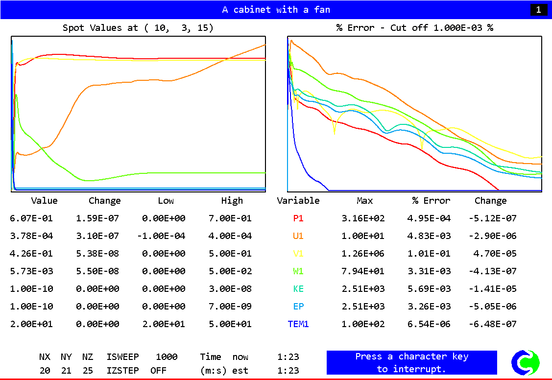
As the Earth solver starts and the flow calculations commence, two graphs should appear
on the screen. The left-hand graph shows the variation of solved variables at the
monitoring point that was set during the model definition. The right-hand graph shows the
variation of errors as the solution progresses.
To the end of the calculation, the monitoring display would be as shown below.
Viewing the results
- Click on the 'Run' button, then on 'Post processor', then 'GUI Post processor (VR
Viewer)' in the FLAIR-VR environment.
- When the 'File names' dialog appears, click 'OK' to accept the current result files. You
may use the 'Object management' dialog box to hide some of objects.
- Click on the 'V' (Select velocity) button,
 followed by the
'Vector toggle' button,
followed by the
'Vector toggle' button,  . You will see the velocity vector displaying on X plane. Moving the
X-position to 0.25m, you will see the following picture on the screen.
. You will see the velocity vector displaying on X plane. Moving the
X-position to 0.25m, you will see the following picture on the screen.
- Click on 'Vector toggle' button to clear the velocity vectors
- Click on 'Slice direction Z' button and move the probe position to Z =0.36
- Click on 'Select temperature' toggle,
 and click on 'Contour toggle' button,
  . To see inside
the chips, switch to wire-frame mode by clicking the wire-frame toggle
. To see inside
the chips, switch to wire-frame mode by clicking the wire-frame toggle
 .The following picture
will appear.
.The following picture
will appear.
- Use 'File' menu and select 'Open file for Editing' and 'Result (output file)' to open
the result file.
- Near the end of the result file, you will find information about the operating point of
your fan-system as follows.
Final result: Operating point data
Operating point data at sweep =   1000

 System mass flow rate:   3.0915E-02 kg/s  1.1130E+02 kg/h

 Fan Name: FAN              Fan Type: FAN1
 FAN              mass flow rate:     3.0916E-02 kg/s   1.1130E+02 kg/h
 FAN              volume flow rate:   2.5671E-02 m^3/s  9.2414E+01 m^3/h
 FAN              velocity:           4.2784E-01 m/s
 FAN              pressure drop:      6.0686E-01 Pa
Saving the case
Once a case has been completed, it can be saved to disk as a new Q1 file by 'File -
Save working files'. The Q1 and associated output files can be saved more permanently by
'File - Save as a case'.