Tutorial 3 Comfort index in a room
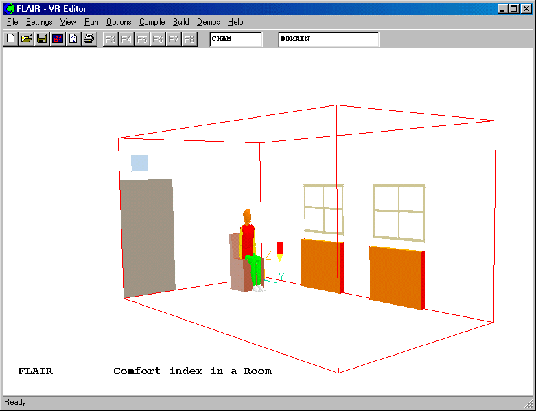
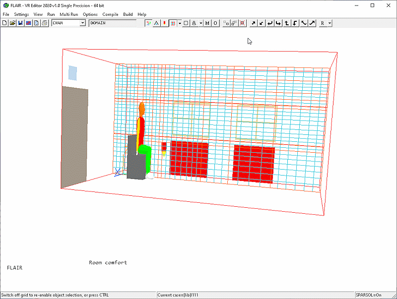
This tutorial is similar to tutorial 2, but with an added person sitting on a chair
as shown in the following figure. The case is to show how to activate the comfort index
calculation.

Setting up the model
Follow the step-by-step instructions for Tutorial 2 in section 6.2.1, from 1. Start
FLAIR with the default room to 3. Adding objects to the room; j. add the
adiabatic walls at the x plane (west). Then we add a sitting person and a chair as
follows.
- Start FLAIR with the default room
The same as for tutorial 2
- Resize the room
The same as for tutorial 2
- Adding objects to the room
a. b. c. d. e. f. g. h. i. j sections are the same as for tutorial 2
k. add a chair
- Click on the 'Object' menu and select 'New' (New Object), 'Blockage' on the 'Object management'
dialog box to bring up the 'Object specification' dialog box
- Change name to 'CHAIR'
- Click on the 'Size' button and set 'Size' of the object as:
X: 0.46 m
Y: 0.39 m
Z: 1.0 m
- Click on the 'Place' button and set 'Position' of the object as:
X: 0.75 m
Y: 0.6 m
Z: 0.0 m
- Click on the 'Shape' button and click on 'Geometry'
- Select 'Chair2s' from d_object/public/furnture and click on 'Save'
- Click on 'OK' to close the 'Object specification' dialog box
- Use the 'Rotate object up' button (located at top of Main Menu),
 to rotate the
CHAIR object until the seat faces the positive y direction.
l. add a sitting person
The PERSON object is used to set the heat source. Its material is the domain material
(air in this case).
- Click on the 'Object' menu and select 'New' (New Object), 'Person' on the 'Object management'
dialog box to bring up the 'Object specification' dialog box
- Click on 'Attributes' and select 'Posture' 'Sitting' and 'Facing' +X.
- Set the total heat source to 50 W and then click 'OK' to close the 'Attributes' dialog
box
- Click on the 'Place' button and set 'Position' of the object as:
X: 0.88 m
Y: 0.74 m
Z: 0.0 m
- Click on 'OK' to close the object specification dialog box
To activate the physical models
a. The Main Menu panel
- Click on the main 'Menu' button.
- Click on the 'Title' dialogue box. Then type in 'Comfort indices in a room'.
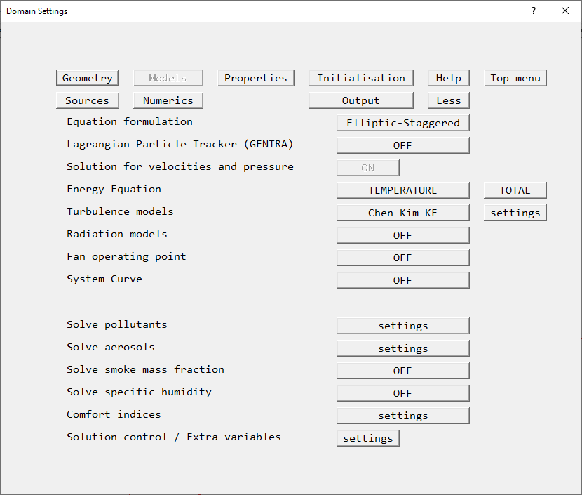
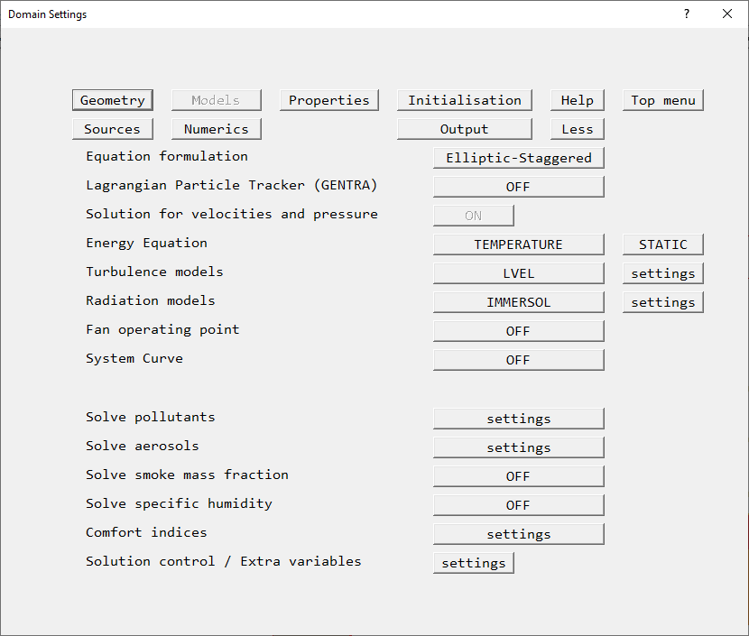
- Click on 'Models' to obtain the Model menu page.
FLAIR always solves pressure and velocities. The temperature is also solved as the
default setting.

The 'Models' page of the Main Menu.
b. To activate LVEL turbulence model
- Click on the 'Turbulence models' button to bring up a list of available turbulence
models. Select the 'LVEL' from it.
- Click on 'OK'.
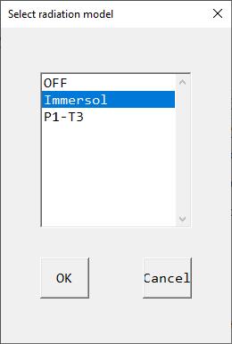
c. To activate IMMERSOL radiation model
- Click on 'Radiation models' button. The following dialog box will appear

- Select 'Immersol' and the click 'OK' to return to the 'Models' panel as shown below

d. To activate Comfort indices
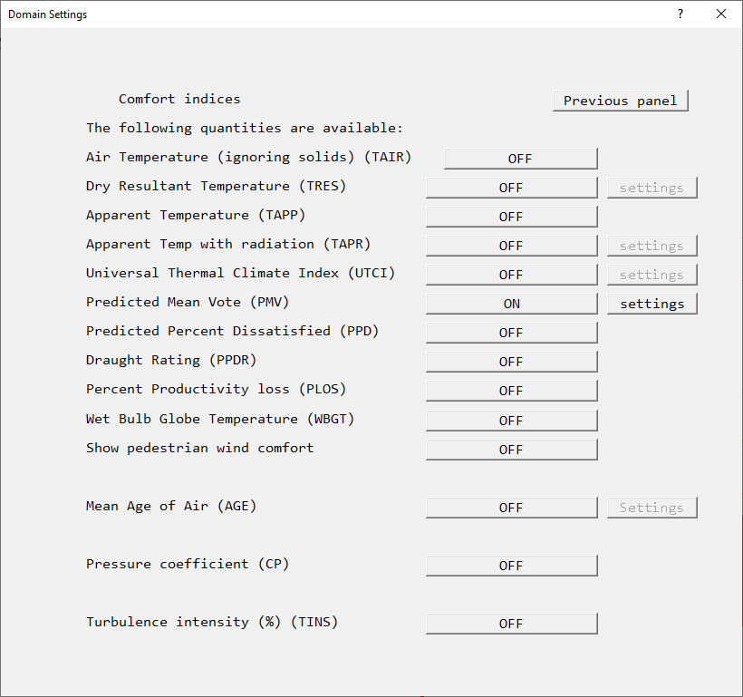
- Locate 'Comfort indices' and then click on its 'Settings' button
- Switch on ' Predicted Mean Vote' (PMV) as shown below. Click 'Settings' and set Radiant temperature to Solved.

- Click on 'Previous panel', followed by clicking on 'Top panel'
To set the grid numbers and to solver parameters
- Click on the Mesh toggle
 on the hand-set or toolbar, then click on the image to bring up
the Grid mesh Settings dialog. The default grid will have 64, 48 and 64 cells in X, Y and Z.
- Click on 'Initialisation', then set the following initial values:
Variable W1
FIINIT Value 0.01
The above initial settings are used to secure the convergence.
- Click on 'Top menu' to return to the top menu
- Click on Main menu, on 'Numerics'
- Click on 'Limits on variables', then set the following values:
Variables T3 TEM1
Minimum value 15 15
The above settings are used to secure the convergence.
- Click on 'Previous panel'
- Click on "Top menu" back to the top menu panel
- Next, a point in the flow domain should be set where the flow variables can be probed or
monitored as the solution runs. The monitor point is shown as the red pencil (probe). It
can be moved interactively with the X/Y/Z position up and down buttons, as long as no
object is currently selected. For example, set the x position =0.67, the y position =1.35m
and the z position =0.44m. It can also be set by clicking on 'Output' on the main menu.
For this case, set the monitor-cell location to (8,14,3).
Running the Solver
To run the PHOENICS solver, Earth, click on 'Run', then 'Solver', then click on 'OK' to
confirm running Earth. These actions should result in the PHOENICS Earth monitoring
screen.
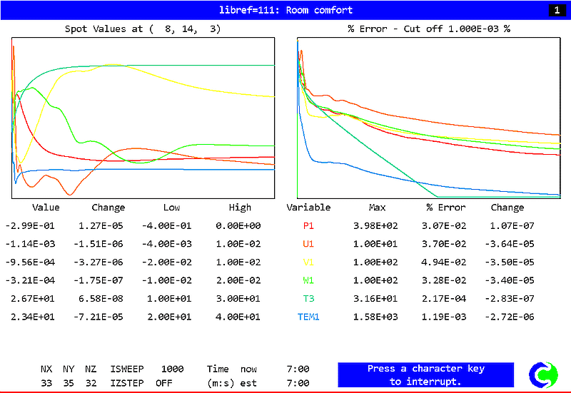
As the Earth solver starts and the flow calculations commence, two graphs should appear
on the screen. The left-hand graph shows the variation of solved variables at the
monitoring point that was set during the model definition. The right-hand graph shows the
variation of errors as the solution progresses.
To the end of the calculation, the monitoring display would be as shown below.
Viewing the results
- Click on the 'Run' button, then on 'Post processor', then 'GUI Post processor (VR
Viewer)' in the FLAIR-VR environment.
- When the 'File names' dialog appears, click 'OK' to accept the current result files. You
may use the 'Object management' dialog box to hide some of objects.
- Click on the 'V' (Select velocity) button,
 followed by the
'Vector toggle'
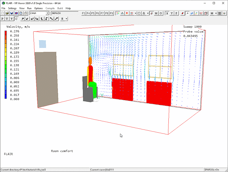
  . You will see the velocity vector displaying on X plane. Move the X-position
to 0.1m near the radiators, and use "Vector option" in the "Settings"
menu to change the scale factor to 0.02. You will see the following picture on the screen.

Velocity vectors at X= 0.1m plane

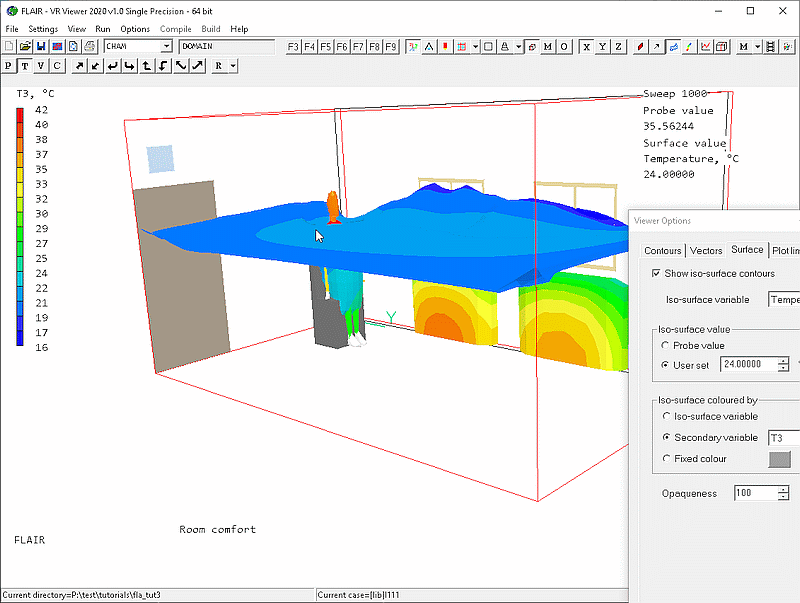
- Click on 'iso-surface toggle' to clear the iso-surface of the temperature contour
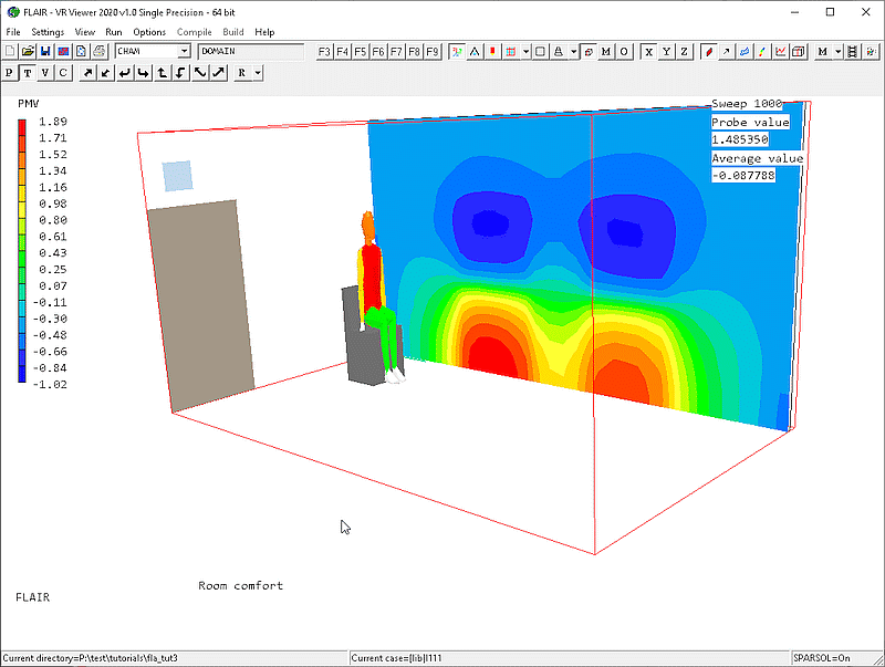
- Click on 'C', 'Select a variable' button, and select 'PMV'. The following figure showing 'Predicted Mean Vote' will
appear on the screen.

The value of predicted PMV is between +1(slightly warm) and -1(slightly cool).
Saving the case
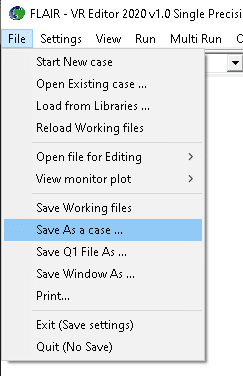
Once a case has been completed, it can be saved to disk as a new Q1 file by 'File -
Save working files'. The Q1 and associated output files can be saved more permanently by
'File - Save as a case'.
