FLAIR Tutorial 10: Fire and Smoke Modeling
This example provides step-by-step instructions on how to activate a FIRE object for a
typical t-squared fire and set the relevant smoke production and visibility parameters. In
the second part of the tutorial, a pair of jetfans is introduced to try to blow the smoke
away from one side of the domain. In the third stage, In-Form is used to modify the
jetfans so that they activate when the temperature at a monitor point rises above a
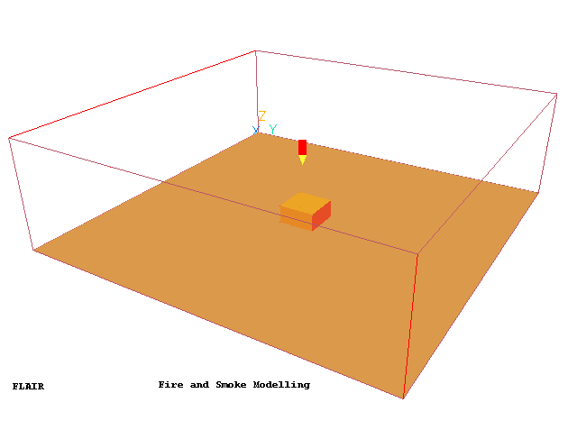
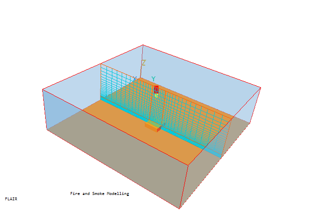
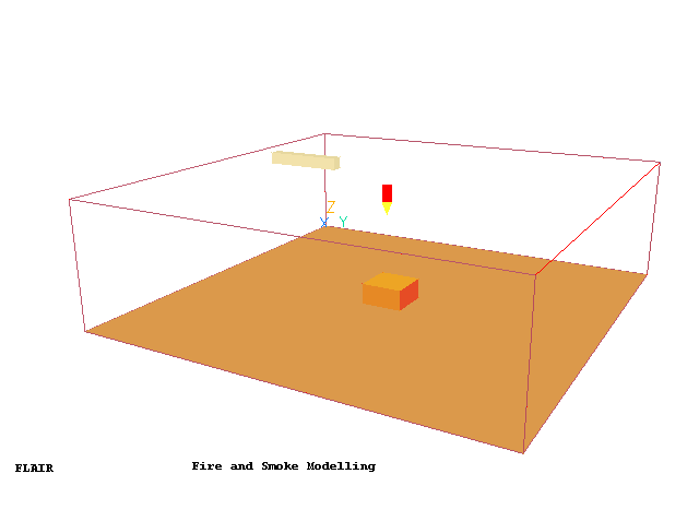
trigger value. The geometry of the case is shown in the figure below.

The size of the domain is 10m long x 10 m wide x 3 m high. A fire is located on the
floor in the middle of the domain. All four vertical faces of the domain are open to
atmosphere.
The fire obeys a t2 law, Q=a.t2, where the a constant is set for
a 'fast' fire as per Table10.1 of the CIBSE Guide E, Fire Engineering. The heat of
combustion, smoke particulate yield and CO yield are set for 'Timber', from Table 10.7 of
CIBSE Guide E.
The entire simulation lasts for 300 seconds.
Setting up the model for stage 1
Start FLAIR with the default mode of operation
To activate the physical models
a. The Main Menu panel
- Click on the 'Main Menu' button. The top page of the main menu will appear on the
screen.
- Click on the 'Title' dialogue box. Then type in 'Fire and Smoke Modeling'.
- Click on 'Geometry' to obtain the Grid Mesh Settings dialog.
- Change 'Time dependence' from Steady to Transient.
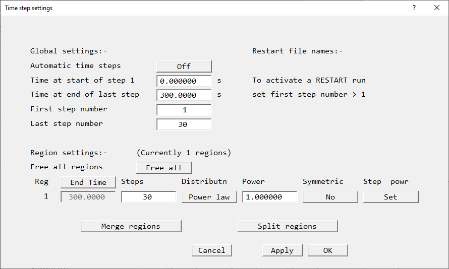
- Click on 'Time step settings' and set the input as shown below

- Click on 'OK' twice to close the 'Geometry' panel.
- Click on 'Models' to obtain the Model menu page.
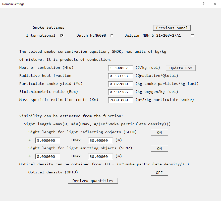
- Switch 'Solve smoke mass fraction' to 'ON' and then 'click on its 'settings'

- Set the Heat of combustion to 1.3E7 J/kg. Click 'Update Rox' to update the
Stoichiometric Ratio.
- The Radiative heat fraction specifies the fraction of the heat released which is
supposed to be transferred by radiation - it is therefore ignored in this calculation. The
CIBSE Guide E recommends a value of 1/3 for this.
- Set the particulate smoke yield to 0.022 kg smoke particles/kg fuel. These values are
recommended by CIBSE Guide E for flaming combustion of timber. The help entries suggest
values for other materials (click the ? in the top-right corner, then click on the item
for which you want help).
- The Mass specific extinction coefficient is a fairly universal constant, so can be left
at the default value.
- Switch both sight lengths on. The panel should now look as shown above.
- Click on 'Previous panel'.
- Click on 'Properties. The ambient temperature is set to 20 degC, and the ambient
pressure to zero relative to 1 atmosphere. These values are fine.
- Click on 'Initialisation'. Click on '>' next to the list of variable names to scroll
sideways until the temperature variable TEM1 is visible. The initial value for temperature
(and pressure P1) are both set to 'ambient', so they will take whatever value is set in
the Properties panel.
- Click on 'Sources'. The reference density is deduced from the ambient conditions set on
the Properties panel. The value is used to calculate the buoyancy force, relative to this
value.
- Click on 'Top menu' and 'OK' to close the main menu.
b. add the FIRE object
- Click on
 on the VR-Editor panel (or the
O icon on the tool bar) to bring up the Object Management Dialog; and then on 'Object',
'New', 'New object', 'Fire'.
- Change 'Name' to 'FIRE'
- Click on the 'Place' button and set 'Position' of the object as:
X: 4.5 m
Y: 4.5 m
Z: 0.0 m
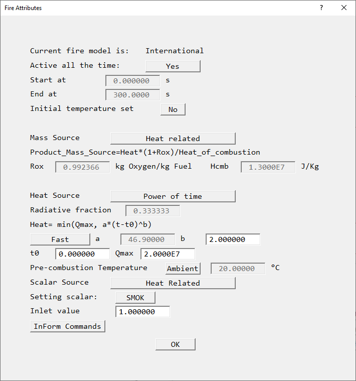
- Click on 'General' and then click on 'attributes'.
- Set the rest of input as shown below. Please refer to section 3.1.2 of TR313 Flair User Guide
for the definition of each entry.

- The value of 46.9 for the 'a' constant is recommended by the CIBSE Guide E for a 'fast'
t-squared fire.
- Click on 'OK' to return to the 'Object management' dialog box.
c. add the floor
- Click on 'Object', 'New', 'New object' 'Plate' and select Z plane on the 'Object management' dialog box to
bring up the 'Object specification' dialog box.
- Change 'Name' to 'FLOOR'
- Click on the 'Size' button and set 'Size' of the object as:
X: tick 'to end'
Y: tick 'to end'
Z: 0.0 m
- Click on 'General' and then 'attributes'.
- Click on 'Adiabatic' next to 'Energy source', and select 'Surface temperature' from the
list. Set the surface temperature to 20C.
d. create the first opening
The four vertical faces of the domain are open to atmosphere.
- Click on 'Object', 'New', 'New object', 'Opening' and select Y plane on the 'Object management' dialog box to
bring up the 'Object specification' dialog box.
- Change 'Name' to 'OPEN1'.
- Click on the 'Size' button and set 'Object size' of the object as:
X: tick 'to end'
Y: 0.0 m
Z: tick 'to end'
- Click on 'General' and then 'attributes'.
- Leave the external pressure and temperature at ambient. Set the external turbulence to
'User set'.
- Click on 'OK' to exit from the object specification dialog.
e. create the remaining openings by copying the first
- Make sure OPEN1 is highlighted in the Object management list.
- Click on the 'Object' pull-down menu and select the 'Copy object' option on the 'Object
management' dialog box. Click OK to allow the OPEN1 object to be copied. A new object will
appear at the bottom of the object list.
- Double-click it to bring up the 'Object specification' dialog box.
- Change 'Name' to 'OPEN2'
- Click on the 'Place' button and set 'Position' of the object as:
X: 0.0 m
Y: tick 'at end'
Z: 0.0 m
- Click on 'OK' to exit from the object specification dialog.
- Make sure OPEN1 is highlighted in the Object management list.
- Click on the 'Object' pull-down menu and select the 'Copy object' option on the 'Object
management' dialog box. Click OK to allow the OPEN1 object to be copied. A new object will
appear at the bottom of the object list.
- Double-click it to bring up the 'Object specification' dialog box.
- Change 'Name' to 'OPEN3'.
- Click on the 'Size' button and set 'Object size' as:
X: untick 'to end' and set 0.0
Y: tick 'to end'
Z: leave 'to end'
- Click on 'OK' to exit from the object specification dialog.
- Make sure OPEN3 is highlighted in the Object management list.
- Click on the 'Object' pull-down menu and select the 'Copy object' option on the 'Object
management' dialog box. Click OK to allow the OPEN3 object to be copied. A new object will
appear at the bottom of the object list.
- Double-click it to bring up the 'Object specification' dialog box.
- Change 'Name' to 'OPEN4'
- Click on the 'Place' button and set 'Position' of the object as:
X: tick 'at end'
Y: 0.0 m
Z: 0.0 m
f. To set the grid numbers and set solver parameters
- Click on the Mesh toggle
 on the hand-set or toolbar, then click on the image to bring up
the Grid mesh Settings dialog. The default grid should look like this and have 48, 48 and 32 cells in X, Y and Z:

- Right click on the mesh and move the 'Minimum cell fraction' slider until there are 28, 28 and 22 cells in X, Y and Z directions respectively. This will happen when the 'Minimum cell fraction' is 2%. The smaller mesh will help the
tutorial run faster.
- Click the mesh toggle again to remove the mesh display.
- Click on the main 'Menu' button and then click on 'Numerics'.
- Change the 'Total number of iterations' to 50.
- Click on 'Relaxation control'. Set U1, V1 and W1 to 0.7. Scroll across the list of variables until temperature
(TEM1) is visible. The maximum increment (MAXINC) for temperature has been automatically
reduced from 1000 deg/sweep to 10 deg/sweep. This gives much better stability when there
are strong heat sources present.
- Click on 'Previous panel', then 'Output'.
- Click on 'settings' of the 'Write flow field' option.
Set 'Intermediate field dumps' to ON, and Step frequency =1.
Set the 'Start letter for solution file', CSG1 to a.
- Click on 'Previous panel' , 'Top menu' and then 'OK'.
g. place the probe
- Click the probe icon
 on the toolbar, then set the probe position to:
X: 5.0
Y: 5.0
Z: 2.0
Running the solver
To run the PHOENICS solver, Earth, click on 'Run', then 'Solver', then click on 'OK' to
confirm running Earth. These actions should result in the PHOENICS Earth monitoring
screen.
NOTE: This will run faster using the 'Run', 'Parallel Solver' option if you have the cores available for this
and your licence allows it.
As the Earth solver starts and the flow calculations commence, two graphs should appear
on the screen. The left-hand graph shows the variation of solved variables at the
monitoring point that was set during the model definition. The right-hand graph shows the
variation of errors as the solution progresses.
Viewing the results
Once the solver has completed step 1 and has started on step2, we can start to plot the
results of step 1.
- Click on the 'Run' button, then on 'Post processor', then 'GUI Post processor (VR
Viewer)' in the FLAIR-VR environment.
- When the 'File names' dialog appears, change 'Use intermediate step files' to 'Yes' and
click 'OK' to accept the result files of step 1.
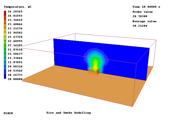
- Click on 'T' (Select temperature) button,
 followed by the 'Contour toggle' button,
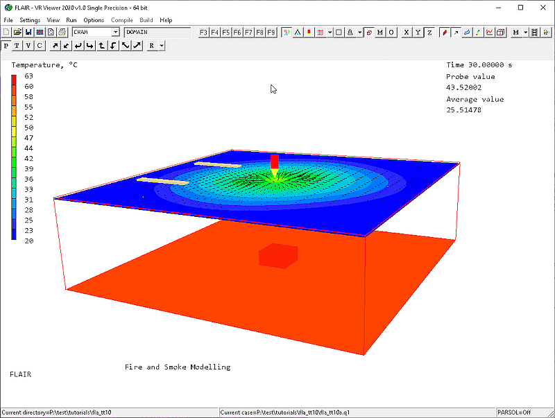
  . The solution after
step 1 should look like this:

- Once the solver run has finished, the solutions can be animated. Click on the 'Run
animation' button,
 . The animation will start, showing the temperature increasing with time.
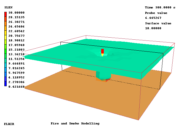
- To see how visibility changes, click on the isosurface toggle
 . Now right-click
the same icon, select SLEN as the variable and set the surface value to 10.

- Regions within the surface have a visibility of < 10m, showing a clear smoke layer by
the ceiling.
Saving the case
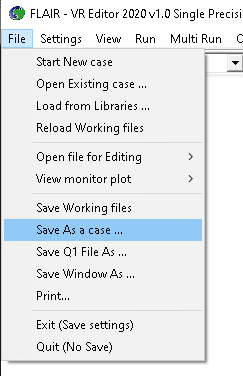
Once a case has been completed, it can be saved to disk permanently by clicking
'File - Save as a case'. Enter 'No fans' as the name of the case, then click Save. Click OK
to save the intermediate step files also. These will be saved to a folder called 'No fans' created in the
current working directory, or wherever the case files were saved.

Setting up the model for stage 2
Adding the jetfans
Jetfans are commonly used in car parks and tunnels to control smoke and air movement.
We will now introduce two jetfans, one on either side of the fire.
h. Create the first Jetfan
- Return to the VR-Editor by clicking Run - Preprocessor - GUI.
- Bring up the Object Management dialog (
 on the VR-Editor panel or the O icon on the tool bar).
- Click on 'Object', 'New', 'New object', 'Jetfan'.
- Change 'Name' to 'FAN1'
- Click on 'General' and then click on 'attributes'.

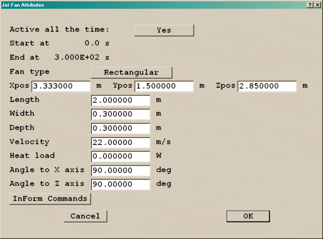
- Set the inputs as shown above. The position boxes set the coordinates of the centre of
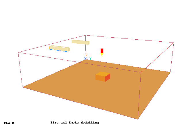
the jetfan. Click 'OK' twice to close the dialogs. The new jetfan should look like this.

i. Create the second Jetfan by copying the first
- Make sure FAN1 is selected in the Object Management Dialog.
- Click on the 'Object' pull-down menu and select the 'Copy object' option on the 'Object
management' dialog box. Click OK to allow the FAN1 object to be copied. A new object will
appear at the bottom of the object list.
- Double-click it to bring up the 'Object specification' dialog box.
- Change 'Name' to 'FAN2'.
- Click on 'General' and then click on 'attributes'. Change Xpos to 6.667 and close
the dialogs. There should now be two jetfans.

Run the solver, then view the results as before. The solution on step 1 should look
like this:

Save the results as a case.
Setting up the model for stage 3
We now want the jetfans to be controlled by a temperature sensor. We want them to
activate when the temperature at (5,5,2.9) reaches 60° C. This can be done by adding an
InForm command to the jetfans.
j. Add the InForm statements
- Select the FAN1 object and double-click it to open its dialog. CLick 'Attributes'.
- Click on 'In-Form Commands'. The Inform Sources dialog will appear.
- Click 'Add Inform'.
- Click the empty button under 'Keyword' and select SOURCE.
- Click the empty button under 'Var' and select V1. The jetfans point along the Y axis, so
it is the V1 velocity which needs to be fixed. If the fans were at an angle to the grid,
both U1 and V1 would have to be fixed appropriately.
- Click the empty button under 'Formula'. An editing window will appear. In the input
window, type
22
then click 'File', 'Save & Exit'.
- Click the empty button under 'Condition'. An editing window will appear. In the
input window, type
if(TEM1{5.0,5.0,2.9}.ge.60)!fixval
then click 'File', 'Save & Exit'. The !fixval condition tells InForm that a fixed
value is to be set. Without this setting, the source would be treated as a fixed flux of
22 Newtons/m3. The InForm sources dialog should now look like this:

Click 'OK' to exit from the In-Form Sources dialog, then 'OK' to exit from the Object
Dialogue Box.
- Repeat the procedure for FAN2.
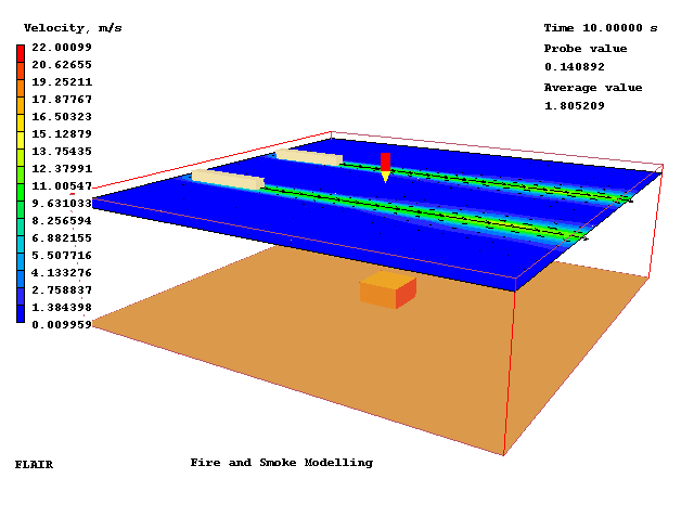
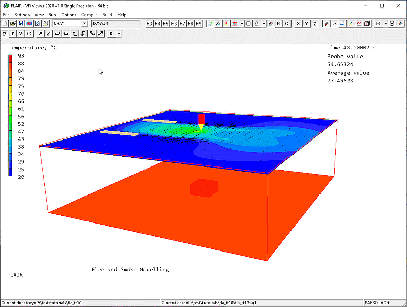
The solver can now be run as before. The solution at step 3 should be:

and on step 4 the jetfans should have activated:

Once again, save the case.
