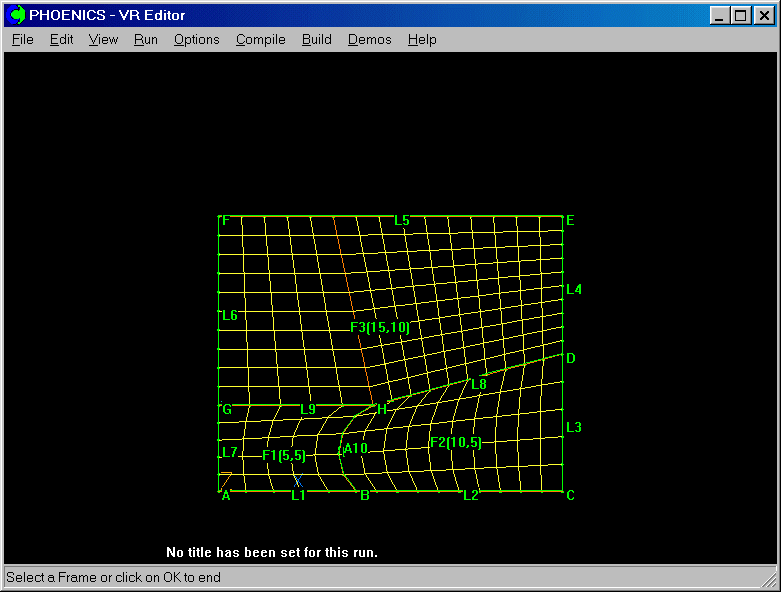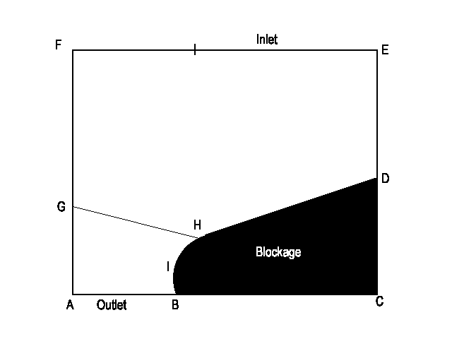
This workshop deals with the creation of a simple BFC grid, sets the flow boundary conditions, and visualises the solution. The case considered is the flow past a non-rectangular blockage, shown here:
All the lines are straight, except line B-I-H, which is an arc.
Three frames will be required. Their corner points will be:
Frame F1 - A, B, H, G
Frame F2 - B, C, D, H
Frame F3 - G, D, E, F
The line G-H is only required for the definition of frame F3, otherwise there would be no connection between G and D.
The co-ordinates of the points can be taken to be:
| Point | Xpos | Ypos | Zpos |
| A | 0.0 | 0.0 | 0.0 |
| B | 0.4 | 0.0 | 0.0 |
| C | 1.0 | 0.0 | 0.0 |
| D | 1.0 | 0.4 | 0.0 |
| E | 1.0 | 0.8 | 0.0 |
| F | 0.0 | 0.8 | 0.0 |
| G | 0.0 | 0.25 | 0.0 |
| H | 0.45 | 0.25 | 0.0 |
| I | 0.35 | 0.125 | 0.0 |
The final outcome of this tutorial is available as Library case B116.
From the system level:
To enter the PHOENICS-VR environment, click on the PHOENICS icon on the desktop, or click on Start, programs, PHOENICS, PHOENICS.
From the commander level:
To enter the PHOENICS-VR environment, click on the 'Run vre' icon in the left column.
In PHOENICS-VR environment,
Start with an 'empty' case - click on 'File' then on 'Start New Case', then on 'Core', then click on 'OK'; to confirm the resetting.
To enter VR Editor:
This is the default mode of operation.
Enter BFC mode by clicking on the Grid Mesh toggle ![]() on the hand-set, then clicking anywhere within the domain to bring
up the 'Grid Mesh Settings' dialog. Click on Coordinate System - Cartesian,
and select Body-fitted.
on the hand-set, then clicking anywhere within the domain to bring
up the 'Grid Mesh Settings' dialog. Click on Coordinate System - Cartesian,
and select Body-fitted.
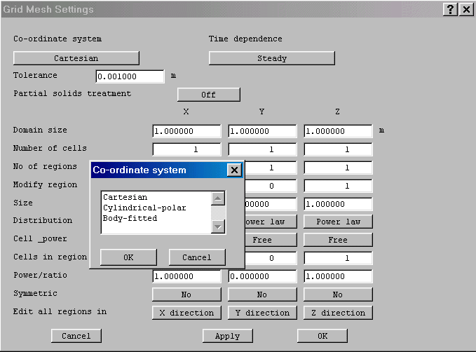
Confirm the change to BFC. Activate the Grid Generator by clicking anywhere in the domain again. A new dialog will appear, overlaid over the hand-set.
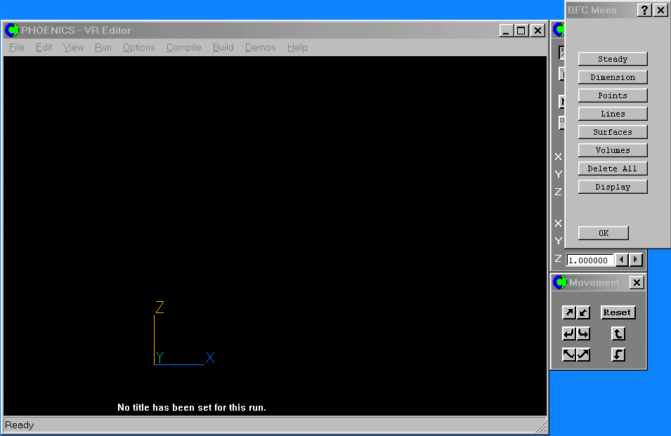
This is the main BFC Menu dialog.
Mesh generation in the Grid Generator
The geometry is to be created on the Cartesian X-Y plane. Click the 'View down' ![]() button on the Movement control panel, and keep it pressed until the view is
more or less along Z, with Y pointing up and X to the right.
button on the Movement control panel, and keep it pressed until the view is
more or less along Z, with Y pointing up and X to the right.
To ensure that the axis orientation is absolutely as desired, click the 'Reset' button on the Toolbar to jump the view to be along the nearest axis (Nearest head on).
Create the points. Click on 'Points', then 'New Points', then 'Type x,y,z'. Enter the co-ordinates of point A as given in the table above. Change the name of the point to A. Click 'Apply' to create the point. Continue for the remaining points. After creating point I, click Cancel to quit the point creation menu. Click 'OK' twice to get back to the main BFC Menu dialog.
Click 'Reset' on the Toolbar, then 'Fit to window' to re-scale the view to fit the geometry.
Create the straight lines. Click on 'Lines', then 'New lines' and then 'New Straights'. Click on A, then B. Line L1 will be created. Now click on B then C to create line L2. Continue with C-D, D-E, E-F, F-G, G-A, D-H and G-H.
Create the arc. Click on 'New Arcs'. Click on B, then I, then H. Arc A10 will be created. Click 'OK' to stop creating arcs.
Set the numbers of cells along each line. Click on 'Modify Lines'. Click on line L1. In the line modification dialog, set the number of cells to 5. Click OK. Click on line L2, and set 10 cells. Continue setting cells as follows:
| Line | Cells |
| L1 | 5 |
| L2 | 10 |
| L3 | 5 |
| L4 | 10 |
| L5 | 15 |
| L6 | 10 |
| L7 | 5 |
| L8 | 10 |
| L9 | 5 |
| A10 | 5 |
Click 'OK' twice to get back to the main BFC Menu dialog.
Set the grid dimension. Click on Dimension, and set NX to 15, NY to 15. This tells the mesh generator how many cells in total it has to set. Click 'OK'.
Create a surface:
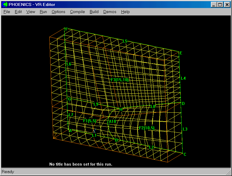
Step 1 - Create the frames. Click on 'Surfaces', then 'New Frames'. Click on points A, B, H , G and A again to close frame F1. Click on points B, C, D, H and B to make frame F2. Click on points G, H, D, E, F and G to make frame F3. F3 has more than four points, so you must indicate which are the corners. When you click on G the second time, it will turn blue. Now click on D to indicate that it is the next corner, then E. The frame will now be made.
Step 2 - Match the frames. Click on 'Match Grid', then on the label of frame F1. The frame matching dialog will be displayed. In the 'match point A to' boxes, set I = 1, J = 1, K = 1. The direction from A -> B is +I, and B -> H is +J, so no changes are required here. Click 'OK' to set the grid in frame F1. Click 'OK' on the Smoothing dialog to close it.
Now click on the label of frame F2. Point B should be matched to I = 6 (number of cells in L1+1), J = 1 and K = 1. The edge directions are again correct, so click 'OK' to set the grid. Click 'OK' on the Smoothing dialog to close it.
Finally click on the label of frame F3. Point G should be matched to I = 1, J = 6 (number of cells in L7+1), K = 1. The edge directions are again correct, so click 'OK' to set the grid. Click 'OK' on the Smoothing dialog to close it.
At this point, the display should look like this:
Click 'OK' twice to get back to the main BFC Menu dialog.
Create the Volume:
So far, the mesh has been created for the K=1 plane. PHOENICS uses a finite-volume mesh, so both faces (K=1, K=2) must be set. Click 'Volumes', then 'Extrude'. Toggle the extrude direction from I to J to K. Change the copy distance DZ from 1.0 to 0.2, then click 'OK' to close the dialog and perform the extrusion.
Click 'OK' twice to get back to the main BFC Menu dialog.
Use the View control buttons to rotate the image, and see both planes of the grid.
Exit the grid generator by clicking 'OK'.
Activate solution of variables.
In the main menu, click on Models. Click on Equation formulation - Elliptic staggered. Select Elliptic GCV and click OK. This selects the GCV Collocated solver, which is very good at dealing with non - orthogonal (distorted) grids.
Leave 'Solution of velocities and pressure' to 'ON'. and use the default KECHEN turbulence model.
Set numerical controls
Click on Numerics, and enter 100 in the 'Total number of iterations' box.
Exit the Main menu by clicking Top Menu, OK.
All the domain-related settings have been made - now set the flow boundary conditions.
Create the blockage.
Click on 'Settings' pull-down menu and then select 'New' and 'New Object'.
Click on 'Size' and 'Place' buttons to set the size and position as:
| IPos | 5 |
| JPos | 0 |
| Kpos | 0 |
| ISize | 10 |
| JSize | 5 |
| KSize | 1 |
Note that in BFC, object positions are set in terms of cell corner, and sizes in terms of cells occupied. Click OK to set the blockage.
Create the inlet at J=16
Click on 'Settings', 'New' and 'New object'.
Set the object position and size as:
| IPos | 5 |
| JPos | 15 |
| Kpos | 0 |
| ISize | 10 |
| JSize | 0 |
| KSize | 1 |
Planar objects have zero thickness in one direction. Click on Type, and select INLET. Click on ATTRIBUTES, and set the Y direction velocity to -2.0. Note that the velocities are specified in the Cartesian co-ordinate system. Click OK to close the Attributes dialog, and OK to close the Object dialog.
Create the outlet at J=0
Click on 'Settings', 'New' and 'New Object'
Set the size and position as follows:
| IPos | 0 |
| JPos | 0 |
| KPos | 0 |
| ISize | 5 |
| JSize | 0 |
| KSize | 1 |
Click on 'General' and set 'Type' to OUTLET.
Click on Attributes, and switch 'External turbulence' to User-set. We need to do this as the exit cuts a vortex - leaving the 'External turbulence' at the default 'In-cell' leads to excessive turbulence levels in the diffuser section. Click OK twice to close the Object dialog.
Create three plates
We now need three plates to provide friction conditions on the insides of the geometry.
Create the first plate at I=15 (the last cell corner in I).
Click on 'Settings', 'New' and 'New Object'.
Set the size and position as:
| IPos | 15 |
| JPos | 5 |
| KPos | 0 |
| ISize | 0 |
| JSize | 10 |
| KSize | 1 |
Click on 'General' and set 'Type' to PLATE.
Click OK to close the Object dialog.
Make the second plate at I=0 by duplication.
Click the Duplicate object or group button and 'OK'.
Move the duplicated object to Ipos=0.
Click the Y size up button on the hand-set until the new plate extends all the way to the top.
Create the third plate at J=15 (the last cell corner in I).
Click on 'Settings', 'New' and 'New Object'.
Set the size and position as:
| IPos | 0 |
| JPos | 15 |
| KPos | 0 |
| ISize | 5 |
| JSize | 0 |
| KSize | 1 |
Click on 'General' and set 'Type' to PLATE.
Click OK to close the Object dialog.
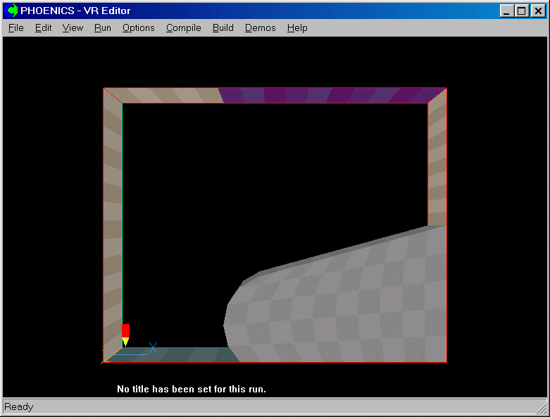
The final geometry should look like this:
Set monitor location
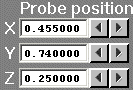
The last action before running the Earth solver is to place the monitoring point (probe) in a sensible location.
Click on the image background, to ensure that no object is active. In this mode, the Position buttons on the hand-set move the probe. Use these to place the probe at (5,10,1).
In the PHOENICS-VR environment, click on 'Run', 'Solver'(Earth), and click on 'OK' to confirm running Earth.
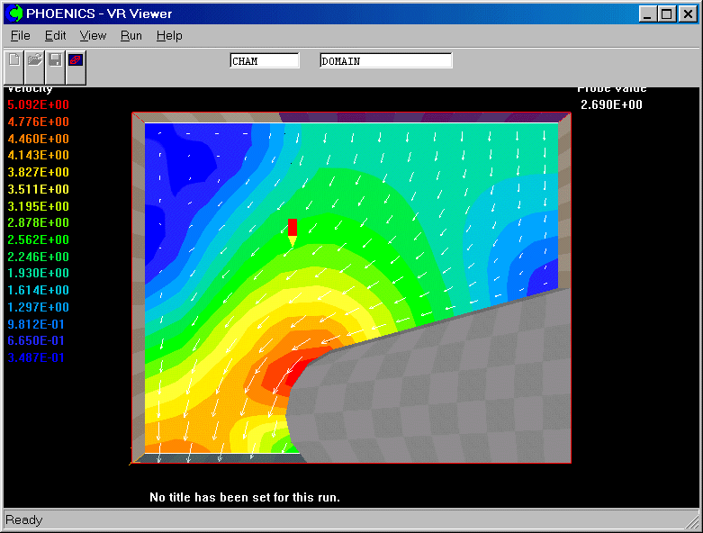
In the PHOENICS-VR environment, click on 'Run', 'Post processor',then GUI Post processor (VR Viewer) . Click 'OK' on the file names dialog to accept the default files.
To view:
To select the plotting variable:
To change the direction of the plotting plane, set the slice direction to X, Y or Z ![]()
To change the position of the plotting plane, move the probe using the probe position buttons
 .
.
In the PHOENICS-VR environment, click on 'Save as a case', make a new folder called 'BFC ' (e.g.) and save as 'CASE6' (e.g.).