The productivity of the reactor depends greatly on the effectiveness of the micro-mixing; but until the arrival of MFMl, there was no practicable way of predicting this.
The prediction problem is complicated by the facts that the geometry is three-dimensional; and unsteady analysis is needed in order to represent properly the effects of the stirring paddle and of the rotation-impeding fixed baffles.
The reactor is one for which the US Dow Corporation has reported experimental data (only hydrodynamic data, alas!) which have been used in "benchmark studies".
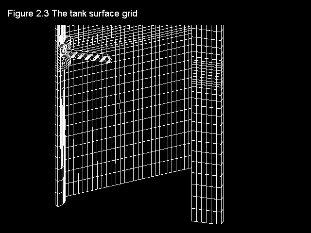
The geometry and computational domain are shown below.
The impeller speed is 500 rpm, the dynamic laminar viscosity is 1.0cP and the water density is 1000 kg/m
The computational grid is divided into two parts, namely an inner part which rotates at the same speed as the impeller, and an outer part which is at rest.
The total number of cells is 31365 (45 vertical, 41 radial and 17 circumferential).
         __________|.|__________
        |          |||          |
        | upper    |.|          |
        | liquid   |||          |
        |          |.|  acid    |
        |..........|||..........|     The paddle-stirred
        | lower    |.| alkali   |         reactor
        | liquid   |||          |
        |       ---------       |
        |paddle /////////       |
        |           .           |
        ------------|------------
                    .< axis of
                       rotation
The sketch illustrates the apparatus and the initial state of the two liquids.
They are both at rest, and are separated by a horizontal interface
The paddle is supposed to be suddenly set in motion.
The computational task is to predict both the macro-mixing, represented by the subsequent distributions of time-average pressure, velocity and concentration, and the micro-mixing, ie the extent to which the two liquids are mixed together at any point.
There is no need, simply because MFM is available, to refrain entirely from using conventional models.
In the present study, therefore, the k-epsilon model was used as the source of the length-scale, effective-viscosity and micro-mixing information.
This allowed the power of the MFM to be concentrated on the process which it alone can simulate, namely micro-mixing and the subsequent chemical reaction.
An eleven-fluid model was employed, with mass-fraction of material from the top half of the reactor (ie the acid) as the population- distinguishing attribute.
This was probably not sufficient to permit achievement of grid-independent of solutions. However, one of the merits of MFM is that population-grid-refinement studies are easily performed.
The simulation procedure therefore generates a very large volume of data, of which only a tiny fraction can be presented here.
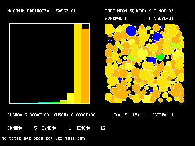
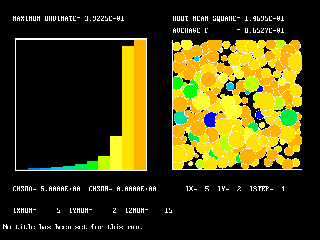
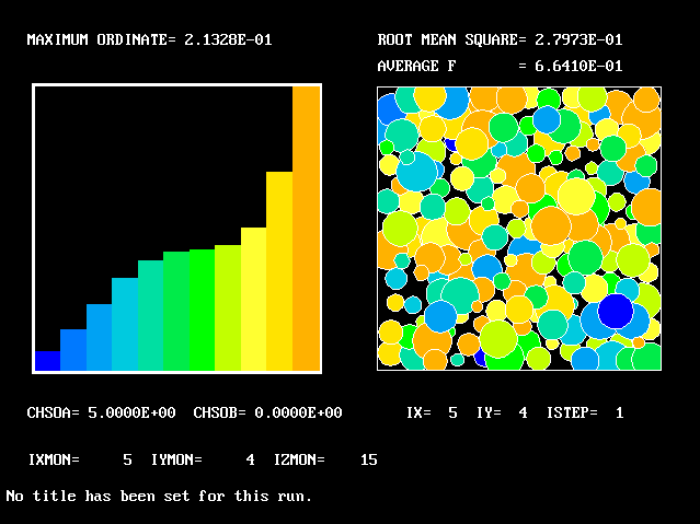
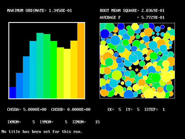
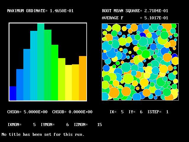
What will first be shown is a series of PDFs. They all pertain to:
Specifically, PDFs will be shown for six radial locations, starting near the axis and moving outward to about one third of the radius.
Near the axis, most of the fluid is still alkaline
Farther from the axis, more-acidic fluids are found
This tendency increases with increase of radius
Also the shape of the PDF changes
This is the last PDF to be shown
The acid and the alkali are supposed to react chemically in accordance with the classic prescription:
acid + base -> salt + water
Of course, no chemical reaction can occur in the unmixed fluids, which (to use the parent-offspring analogy) are the Adam and Eve of the whole population. It is only their descendants, with both acid and alkali "in their blood", who can produce any salt.
This is why the prediction of the yield of salt necessitates knowledge of the concentrations of the offspring fluids.
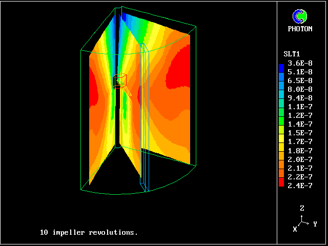
The next picture shows the salt concentrations after 10 paddle rotations which the multi-fluid model has predicted.
These concentrations are the averages for all eleven fluids.
The salt concentrations predicted by the multi-fluid model
They are greatest in the region which has been most vigorously stirred by the paddle, which tends to thrust fluid downwards and outwards.
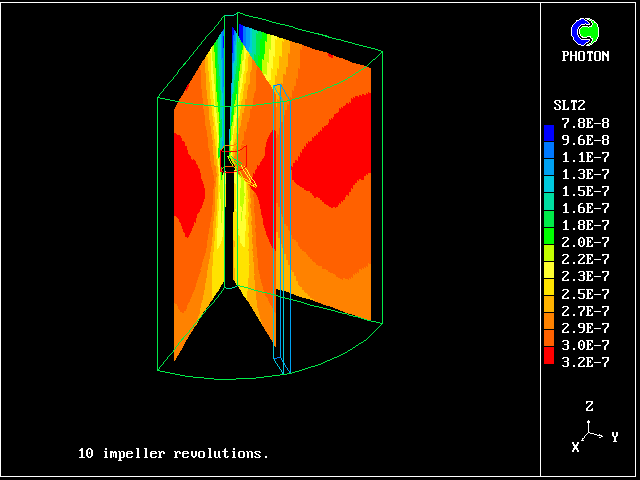
If no account is taken of the existence of the fluctuations, as is perforce the usual case, only the mean value of the acid/base ratio is available.
If the salt-concentration distribution is calculated from this, as the next picture will show, the values will be different from before.
Indeed it can be expected that they will be larger, because the implication of using a single-fluid model (which is what neglect of fluctuations amounts to) is that micro-mixing is perfect.
This is indeed what is revealed by the calculations.
The salt concentrations predicted by the single-fluid model
They are larger than the multi- fluid values, because micro- mixing is presumed (wrongly) to be perfect.
The following conclusions appear to be justified by the studies conducted so far:-