abstract or contents or update

Abstract

• It is often believed that fluid-flow and solid-stress problems must be solved by different methods and different computer programs.

• This is not true, if the solid-stress problems are formulated in terms of displacements.

• The lecture exemplifies and explains how both displacements and velocities can be calculated at the same time.

next











This is not the only common fallacy that will be exposed. Specifically:

1. It is often believed that thermal radiation between solids separated by non-participating gases must be computed by view-factor or ray-tracing techniques.

   But:

   • These become hopelessly expensive when many solids are present, as in a furnished room or an engine compartment; and

   • it is not true because the IMMERSOL conductivity-type method handles the problem inexpensively and well.

   next
   
   
   
   
   
   
   
   
   
   
   
   

2. It is often believed that convective heat transfer at low Reynolds number, which prevails for example in electronics equipment, requires an advanced 2-or-more-differential equation model for its prediction.

   However:

   • these are also computationally expensive; and

   • the no-differential-equation LVEL model does just as well at much lower cost.

   next
   
   
   
   
   
   
   
   
   
   
   
   

3. Both kinds of turbulence model require knowledge of the "distance from the wall", and sometimes "distance between walls"; and it is often believed that complicated trigonometrical computations must be conducted so as to acquire it.

   However:

   • these are expensive as well as complicated; and

   • they are also not needed, because the easy-to-solve LTLS equation provides all that is needed at negligible cost.

next











To summarise, four misconceptions are to be dispelled, namely that:

1. solid-stress analysis needs a separate program;

2. solid-to-solid radiation needs view-factors or ray tracing;

3. low-Re convection needs (e.g.) Lam-Bremhorst;

4. wall-distance computation requires trigonometry.

next or back

Contents

1. The problem
   1. Its essential nature
   2. Practical occurrence
   3. The conventional solution
   4. A better solution

2. A multi-physics example
   1. Stresses resulting from radiation, conduction and convection
   2. Vector and contour plots
   3. How the stress calculations were performed

   next or back or contents
   
   
   
   
   
   
   
   
   
   
   
   

3. The mathematics of the method
   1. Similarities between the equations for displacement and velocity
   2. Deduction of the associated stresses and strains
   3. The "SIMPLE" algorithm for the computation of displacements
   4. More details of the equations

4. Details of the auxiliary models
   1. IMMERSOL, for radiation
   2. WGAP, WDIS and LTLS, for radiation and turbulence
   3. LVEL, for turbulence

5. Discussion of achievements and future prospects

6. References

next or back or contents

1. The problem

It is frequently required to simulate fluid-flow and heat-transfer processes in and around solids which are, partly as a consequence of the flow, subject to thermal and mechanical stresses.

Often, indeed, the stresses are the major concern, while the fluid and heat flows are of only secondary interest.

next, back or contents











(b) Practical occurrence

Engineering examples of fluid/heat/stress interactions include:

• gas-turbine blades under transient conditions;

• "residual stresses" resulting from casting or welding;

• thermal stresses in nuclear reactors during emergency shut-down;

• manufacture of bricks and ceramics;

• stresses in the cylinder blocks of diesel engines;

• the failure of steel-frame buildings during fires.

(c) The conventional solution

It has been customary for two computer codes to be used for the solution of such problems, one for the fluid flow and the other for the stresses

Iterative interaction between the two codes is then employed, often with considerable inconvenience.

next, back or contents

(d) A better solution

It is however possible for fluid flow, heat flow and solid deformation, and the interactions between them, all to be calculated at the same time.

The method of doing so exploits the similarity between the equations governing velocity (in fluids) and those governing displacement (in solids).

In the present lecture, the results of such a calculation will be shown first.

The explanation of how it was conducted will then follow.

next, back or contents

2. A multi-physics example

The task is to calculate the stresses in radiation-heated solids cooled by air.

    20 deg C| air
            |             80 deg C
          | V |/////// hot radiating wall ///////////|
          |   ----------------------------------------
          |                       duct              ----->  exit
          |-------------                 -------------
          |// copper //|     cavity      |//copper //|
          |------------------------------------------- ? temperature ?
          |////////////// aluminium /////////////////|
          |-------------------------------------------

Details of the calculation are:

1. The Reynolds number (based on the inflow velocity and horizontal duct width) is 1000.
   Therefore the LVEL model is used for simulation of the turbulence.

2. The radiative heat transfer is represented by the conduction-type IMMERSOL model, which is:
   1. economical and
   2. fairly accurate
   for such situations.

   The absorptivity of the air is taken as 0.01 per meter;
   the scattering coefficient as 0.0;
   and the solid surface emissivity as 0.9 .

   next, back or contents
   
   
   
   
   
   
   
   
   
   
   
   

3. Both LVEL and IMMERSOL make use of the distributions of:
   1. distance from the wall (WDIS) and

   2. distance between walls (WGAP), both of which are calculated by solving a scalar equation for the

   3. LTLS variable.

4. The stresses within the metals result primarily from the differences in their thermal-expansion coefficients. namely:
   • 2.35 e-5 for aluminium, and

   • 1.67 e-5 for copper.

next, back or contents

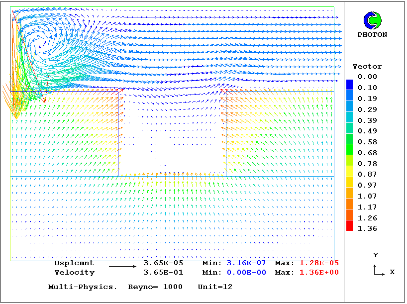
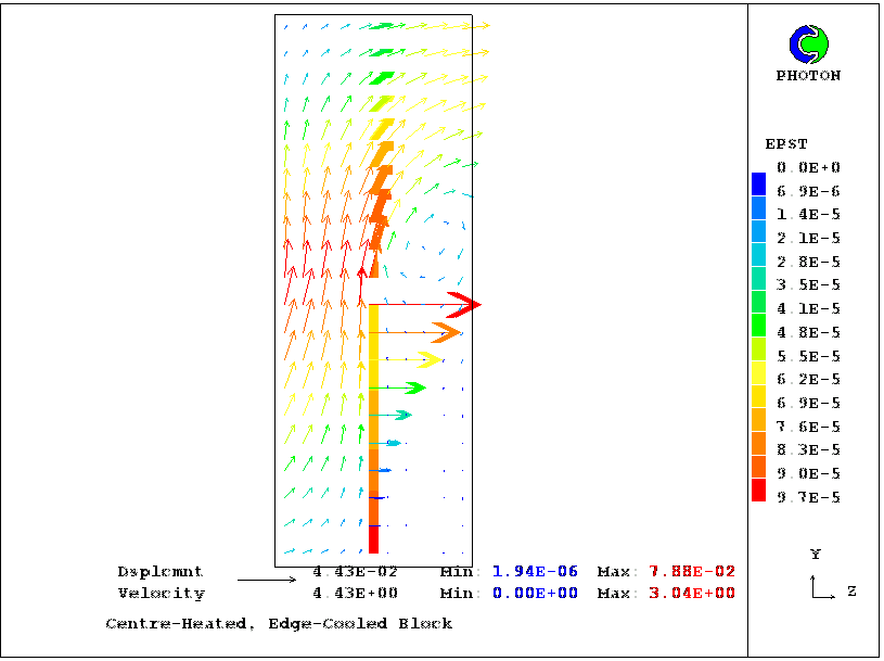
(b) Vector and contour plots

• Vectors

  The vectors displayed in Fig.1 show simultaneously:

  1. the nature of the air-flow pattern (upper part of the domain), and
  2. the displacements of the solid material (lower part of the domain).

  Both are calculated at the same time. Of course, the two sets of vectors have different scales, and indeed dimensions. namely m/s for velocity and m for displacements.

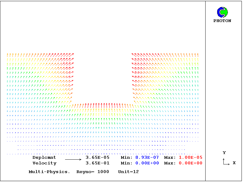
  The displacement vectors are shown on their own in Fig. 1a

  next, back or contents
  
  
  
  
  
  
  
  
  
  
  
  

  The solids are supposed to be confined by a stiff-walled box, but are allowed to slide relative to its walls. This is why the displacement vectors are vertical near the confining-box walls.

  They are however not allowed to slide relative to each other; this is what causes the concentrations of stress at their contact surfaces.

  next, back or contents
  
  
  
  
  
  
  
  
  
  
  
  

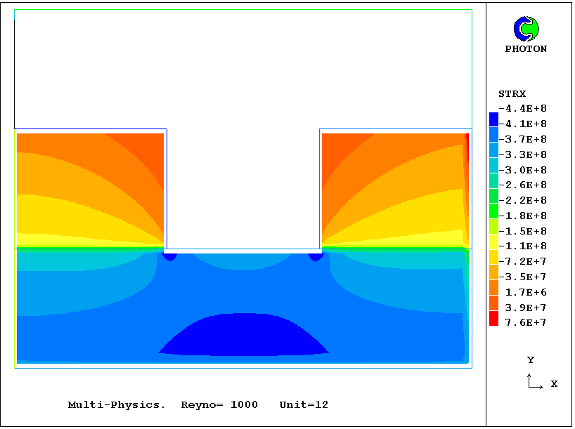
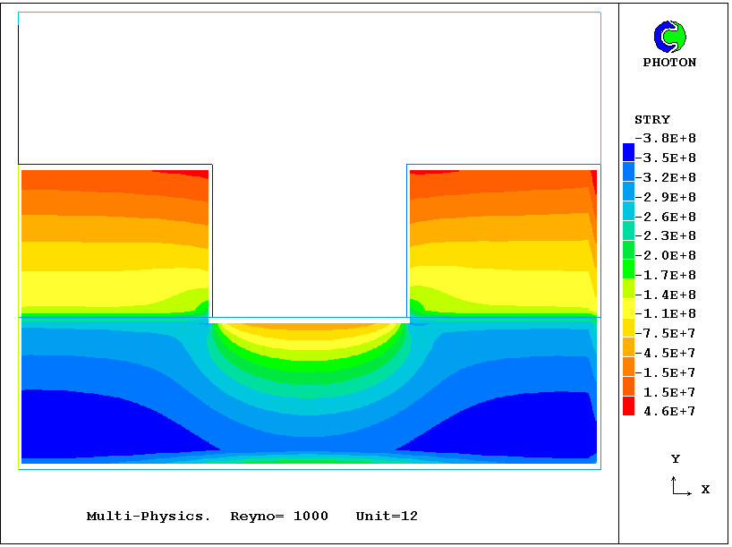
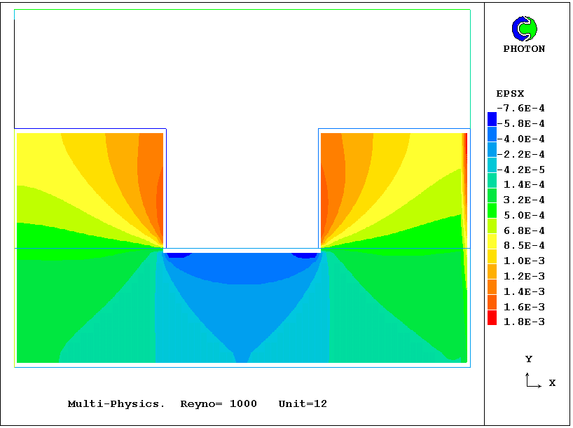
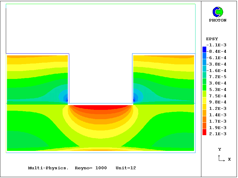
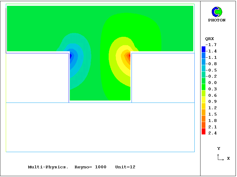
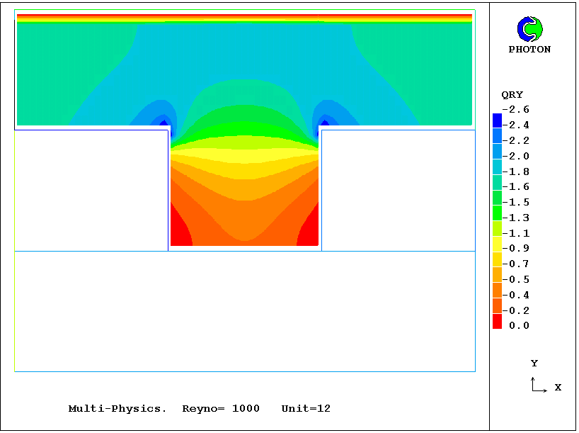
• Stresses and strains

  The stresses in the x- (horizontal) and y- (vertical) directions are displayed in Fig.2 and Fig.3 respectively.

  They have been deduced from the strains shown in

  Fig.4 for the x-direction , and in

  Fig.5 for the y-direction,

  next, back or contents
  
  
  
  
  
  
  
  
  
  
  
  

  The strains have been deduced from the displacements by differentiation. The displacements are however not here displayed as contour plots because these do not easily display small variations.

  That is the end of the stress-strain results.

  There will now be shown some of the other variables which had to be computed.

  next, back or contents
  
  
  
  
  
  
  
  
  
  
  
  

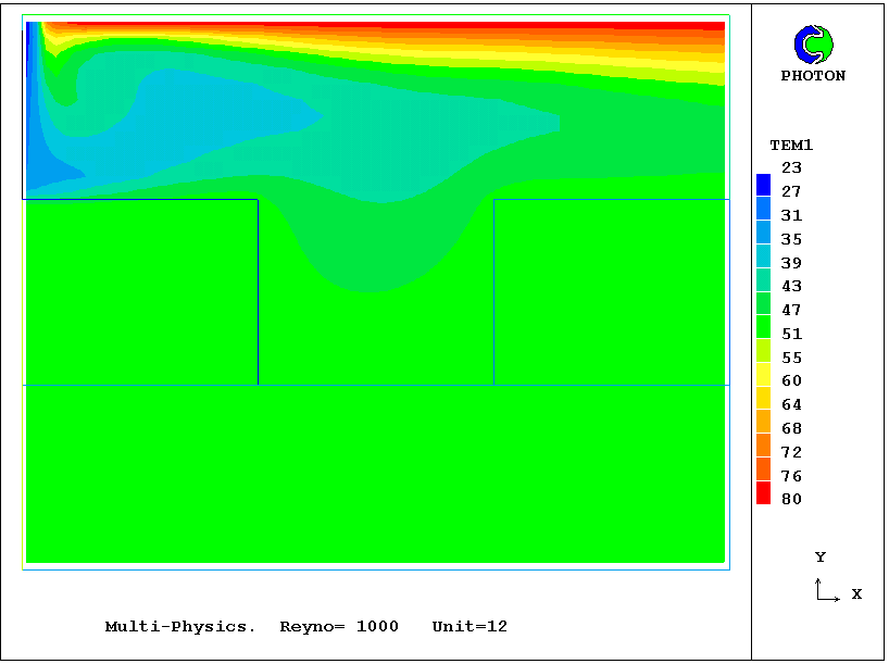
• Temperature fields

  Fig. 6 displays contours of temperature in the air and the solid, and reveals that:

  • the air is heated by contact with:
    1. the 80-degree-Celsius top wall, and
    2. the metal blocks, which have been receiving heat by radiation from the top wall;

  • temperature differences within the high-conductivity solids are too small to be discerned visually.

  next, back or contents
  
  
  
  
  
  
  
  
  
  
  
  

  It is interesting to compare Fig. 6 with Fig. 7.

  This displays the distribution within the air space of:

  • the "radiation temperature", T3, which:

  • is computed by IMMERSOL, and

  • is defined as the temperature which would be taken up by a probe which was affected only by radiation.

  Obviously, and understandably, T3 and TEM1 have very different values, unless the absorptivity is very great (as in solids).

  next, back or contents
  
  
  
  
  
  
  
  
  
  
  
  

  The solid temperature influences the stresses and strains, of course, primarily through the agency of the temperature-dependent thermal-expansion distribution.

  However, its variations with position, within a single material, are too slight to be revealed by a contour diagram, as inspection of Fig. 8 will reveal.

  next, back or contents
  
  
  
  
  
  
  
  
  
  
  
  

• Radiation-flux contours

  The IMMERSOL model, of which the solution of the T3 equation is the major feature, enables the radiant heat fluxes in the coordinate directions to be established by post-processing.

  The results are displayed in
  Fig. 9 for the x-direction. and by
  Fig. 10 for the y-direction.

  The values and patterns displayed, if studied and interpreted in physical terms, will be found to be plausible.

  Where calculation by hand is easy, namely for the parallel surfaces, they will be found to be correct.

  next, back or contents
  
  
  
  
  
  
  
  
  
  
  
  

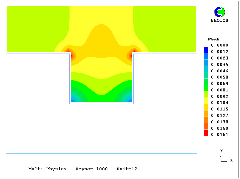
• Contours of auxiliary quantities used by IMMERSOL

  A crucial feature of the IMMERSOL model is its use of the distribution of the "distance between the walls", WGAP.

  This quantity, which has an easily-understood meaning when the walls are near, and nearly parallel, is computed from the solution of the "LTLS" equation;
  this will be explained later in the lecture.

  The distributions of these two quantities are shown by

  Fig. 11 for the former, and by

  Fig. 14 for the latter.

  next, back or contents
  
  
  
  
  
  
  
  
  
  
  
  It will be seen that WGAP has a uniform value in the region of between the top of the duct and the tops of the upper metal slabs, between which the actual distance is 0.008 meters.

  Further, it has approximately twice this value near the convex corners; and it becomes zero in the concave corners.

  next, back or contents
  
  
  
  
  
  
  
  
  
  
  
  

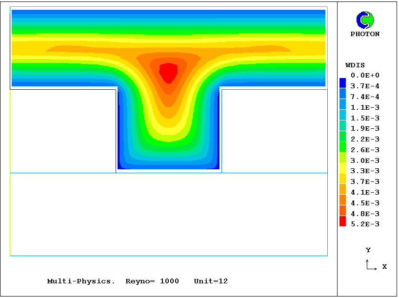
• Contours of auxiliary quantities used in the fluid-flow calculation

  The flow field was calculated by means of the LVEL turbulence model, which makes use of the wall-distance (WDIS) field.

  This, like WGAP, is also derived from the LTLS distribution.

  The contours of WDIS are displayed in Fig. 13.
  which exhibits:

  • the expected maximum of 0.004 between the parallel horizontal walls, and
  • a somewhat greater value near the cavity, where the true distance from the wall depends on the direction in which it is measured.

  next, back or contents
  
  
  
  
  
  
  
  
  
  
  
  

  LVEL, like IMMERSOL, is a "heuristic" model, by which is meant that it is incapable of rigorous justification, but is nonetheless useful.

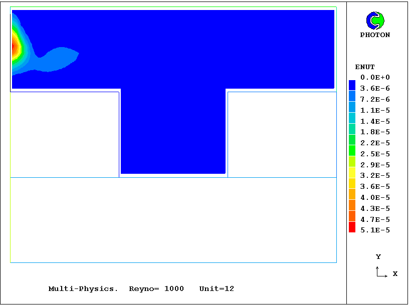
  WDIS is calculated once for all, at the start of the computation. From it, and from the developing velocity distribution, the evolving distribution of ENUT, the effective (turbulent) viscosity is derived.

  The resulting contours of ENUT are shown in Fig. 14.

  Since the laminar viscosity is of the order of 1.e-5 m**2/s, it is evident that turbulence raises the effective value, far from the walls, by an order of magnitude.

next, back or contents

(c) How the stresses were calculated

• As will be shown below, the equations governing the displacements are very similar to those governing the velocities.

• The CFD code PHOENICS, like many others, can calculate velocities in fluids; but this ability is not needed in the solid region; so such codes are usually idle there.

• However, PHOENICS can be "tricked" into calculating what it "thinks" are velocities everywhere; whereas what it actually calculates in the solid regions are displacements.

• The details of the "trickery" now follow.

next, back or contents

3. The mathematics of the method

(a) Similarities between the equations for displacement and velocity

The similarities already referred to are here described for only one cartesian direction, x; but they prevail for all three directions.

next, back or contents

1. The x-direction displacement, U, obeys the equation:

   [del**2]* U + [d/dx]* [ D*C1 - Te*C3 ] + Fx*C2 = 0

   where:

   • Te = local temperature measured above that of the un-stressed solid in the zero-displacement condition, multiplied by the thermal-expansion coefficient;

   • D = [d/dx]* U + [d/dy]* V + (d/dz]* W
     which is called the "dilatation";

   • Fx = external force per unit volume in x-direction;

   • V and W = displacements in y and z directions;

   • C1, C2 and C3 are functions of Young's modulus and Poisson's ratio.

   next, back or contents
   
   
   
   
   
   
   
   
   
   
   
   

   • When the viscosity is uniform and the Reynolds number is low, so that convection effects are negligible, the x-direction velocity, u, obeys the equation:
     [del**2]* u - [d/dx]* [ p*c1 ] + fx*c2 = 0 ,

     
     where

     • p = pressure,
       
     • fx = external force per unit volume in x-direction,
       
     • c1 = c2 = the reciprocal of the viscosity.

next, back or contents

Notes:

1. The two equations are now set one below the other, so that they can be easily compared:

   • [del**2]* U + [d/dx]* [ D*C1 - Te*C3 ] + Fx*C2 = 0

   • [del**2]* u - [d/dx]* [ p*c1 ] + fx*c2 = 0 ,

2. The equations can thus be seen to become identical if:
   • p*c1 = D*C1 - Te*C3
     which implies:

     D = [p*c1 + Te*C3 ] / C1

   • and

     fx * c2 = Fx * C2

   next, back or contents
   
   
   
   
   
   
   
   
   
   
   
   

3. The expressions for C1, C2 and C3 are:
   • C1 = 1/(1 - 2*PR)

   • C2 = 2*(1 + PR) / YM

     where

     • PR = Poisson's Ratio. and
     • YM = Young's Modulus

     and

   • C3 = 2 *(1 + PR)/(1 - 2*PR)

   next, back or contents
   
   
   
   
   
   
   
   
   
   
   
   

4. A solution procedure designed for computing velocities will therefore in fact compute the displacements if:
   1. the convection terms are set to zero within the solid region: and

   2. a suitable linear relation between:
      • D ( ie [d/dx]* U + ...)

        and

      • p
      is introduced by inclusion of a pressure- and temperature-dependent "mass-source" term.

next, back or contents

(b) Deduction of the associated stresses and strains

The strains (ie extensions ex, ey and ez) are obtained from differentiation of the computed displacements.

Thus:

ex = [d/dx]* U

ey = [d/dx]* V

ez = [d/dx]* W

next, back or contents

Then the corresponding:

• normal stresses, sx, sy, sz, and
• shear stresses tauxy, tauyz, tauzx,

sx = {YM / (1 - PR**2)} * {ex + PR*ey} and

tauxy = {YM / (1 - PR**2)} * {0.5 * (1 - PR)*gamxy}

where:

• gamxy = [d/dy]*U - [d/dx]*V

next, back or contents

(c) The "SIMPLE" algorithm for the computation of displacements

Its essential features are:

• All the velocity equations are solved first, with the current values of p.

• The consequent errors in the mass-balance equations are computed.
• These errors are used as sources in equations for corrections to p.

• The corresponding corrections are applied, and the process is repeated.

next, back or contents

All that it is necessary to do, in order to solve for displacements simultaneously, is, in solid regions, to treat the dilatation D as the mass-source error and to ensure that p obeys the above linear relation to it.

Therefore a CFD code based on SIMPLE can be made to solve the displacement equations by:

1. eliminating the convection terms (ie setting Re low); and
2. making D linearly dependent on p and temperatureT.

The "staggered grid" used as the default in PHOENICS proves to be extremely convenient for solid-displacement analysis; for the velocities and displacements are stored at exactly the right places in relation to p.

next, back or contents

4. Details of the auxiliary models

(a) IMMERSOL: summary

• The solved differential equation is:
  div( effective_conductivity * T3 ) + source = 0

• effective conductivity =
  0.75 * sigma * T3**3 / (abso + scat + 1/WGAP)

• source = abso * sigma * ( T1**4 - T3**4 )

• in solids, abso = large, so T3 --> T1

• surface resistances account for non-unity emissivities

next, back or contents











Notes:

• The main novelty is the inclusion of WGAP, ie the distance between the walls, in the formulae.

• This enables a conduction-type model to be used even with non-participating media.

• Of course, an economical means of calculating WGAP is needed.

• This is provided by the LTLS equation (see below).

• IMMERSOL gives quantitatively correct predictions in geometrically simple circumstances and plausible ones in complex ones.

• It is economical enough to be generalised for wavelength-dependent radiation.

next, back or contents

(b) WGAP, WDIS and LTLS

• The solved differential equation is:
  div (grad LTLS) = 1

• The boundary conditions are:
  LTLS = 0 , in all solids.

• The solution for plane channel flow is:
  LTLS = WDIS * ( WGAP - WDIS ) / 2 , and
  grad LTLS = WGAP / 2 - WDIS

• These relations are supposed to prevail also in two- and three-dimensional circumstances.

• That is all!

next, back or contents











Notes:

• The LTLS equation is very simple, and therefore easy to solve.

• Its solution yields values of LTLS and grad LTLS at all points in the field.

• WDIS and WGAP are then deduced from them.

• Their values are quantitatively correct predictions in geometrically simple circumstances and plausible in complex ones.

• The method is especially useful, indeed the only practicable one, when the space in question contains many solids of arbitrary shapes.

next, back or contents

(c) LVEL: summary

• LVEL generalises a continuous formula for the "law of the wall", namely:

  
       y+ = u+ + (1/E) * [ exp(K*u+) - 1 - K*u+ -
            (K*u+)**2/2  - (K*u+)**3/6 - (K*u+)**4/24 ]

  which implies another for dimensionless effective viscosity, namely:

  
       v+ = 1 + (K/E) * [ exp(K*u+) - 1 -
            K*u+ - (K*u+)**2/2 - (K*u+)**3/6 ]

  next, back or contents
  
  
  
  
  
  
  
  
  
  
  
  

• These relations enable the effective viscosity to be calculated at every point for which are known:
  • the distance from the wall, y
  • the fluid velocity, u, and
  • the kinematic viscosity

• They are known at all points; so the model is complete.

• The LVEL model presumes that the same relation holds, regardless of the geometry of the solid surface.

• That is all!

next, back or contents











Notes:

• The LVEL model is very simple, and therefore easy to implement.

• The predicted effective viscosities are quantitatively correct in geometrically simple circumstances and plausible in complex ones.

• The method is especially useful, indeed often the only practicable one, when the space in question contains many solids of arbitrary shapes.

• LVEL handles the complete Reynolds-number range: laminar, transitional and fully turbulent.

• LVEL can be easily extended so as to improve its accuracy in locations far from walls.

next, back or contents

5. Discussion of current achievements and future prospects

(a) Preliminary conclusions

The following conclusions appear to be justified:

1. Simultaneous simulation of solid-stress, heat transfer and fluid flow is indeed practicable and economical.

2. As compared with the alternative, namely the use of distinct methods for each phenomenon with iterative interaction between them, the simultaneous-solution method is very attractive.

3. It therefore seems possible that, when its attractiveness is fully recognised, SFT (i.e. Solid-Fluid-Thermal) analysis may become as popular as CFD.

next, back or contents

(b) Why has this recognition not already become widespread ?

1. First, it requires long-held convictions to be questioned and then abandoned. Many people find this uncomfortable.

2. Secondly, those who are in principle willing to try new methods prefer to do so only after very many others have led the way.

   "Never do anything first" commends itself to those who have observed how seldom pioneers actually prosper.

   next, back or contents
   
   
   
   
   
   
   
   
   
   
   
   

3. Thirdly, in the present case, The pioneers ( the author and his colleagues) have been reprehensibly backward in documenting, illustrating and generally promoting the SFT method.

   True: it has been a part of the PHOENICS package for several years, but with too many limitations to be easily usable; and finally

4. The method described above has proved to have two deficiencies, namely:
   1. the SIMPLE algorithm converges rather slowly when both the flow and solid-stress situations are complex and intertwined; and

   2. additional 'source terms' must be provided in order that 'bending' phenomena can be properly represented.

   How to overcome these deficiencies will now be described.

next, back or contents

The better algorithm; revival of an old trick

Mathematical aspects Click here for full details

1. Differentiate:
   the U-displacement equation with respect to y and :
   the V-displacement equation with respect to x.

2. Subtract one from the other, causing the dilatation and thermal-expansion terms to disappear.

3. Hence obtain an easy-to-solve transport equation for the z- direction component of vorticity (the CFD word) or rotation (the stress-analyst's word) k of the form:

   [del**2]*k + K*C2 = 0

   where:
   k = dU/dy - dV/dx and K = dFx/dy - dFy/dx

   next, back or contents
   
   
   
   
   
   
   
   
   
   
   
   

4. Do the same for the V- and W- equations and for the W - and U- equations, thus obtaining equations for the other two vorticity (i.e. rotation) components, i and j.

5. Differentiate the definition of the displacement, D with respect to x, y and z, and thence obtain 3 expressions (only 1 is shown) for its gradients, of the following form:

   dD/dx = [del**2]*U + dj/dz - dk/dy

6. Finally, by algebraic manipulation, derive second-order differential equations for U, V and W of the form:

   [del**2]* U + [dj/dz - dk/dy]*C4 +[d/dx]* [- Te*C3 ] + Fx*C2 = 0

   which is simpler than the earlier equation for [del**2]* U because [dj/dz - dk/dy] is known from the solution for vorticity.

next, back or contents

New solution procedure

1. First solve the three (linear, Poisson-type) equations for the vorticity components.

   Often analytical solutions will suffice.

2. Solve the three (linear, Poisson-type) equations for the displacements (in solids) and velocities (in fluids), which are now linked only at the solid-fluid boundaries.

3. Iterate as necessary, but many fewer times than for pressure-linked equations (i.e. SIMPLE/SIMPLEST).

4. The results of such a calculation can be seen here, where the bending of the beam is clearly visible.

Click here for more details.

next, back or contents

Present stage of development

• The new algorithm has been found to 'converge' much more rapidly than the old.

• If appropriate expressions for 'vorticity sources' (I, J and K) are introduced so as to express the 'bending moments' exerted by the applied forces, bending phenomena are well simulated.

• The forces exerted by the fluid on the solid are easily taken into account they are calculated simultaneously.

• There appear to be no difficulties of principle in the way of extension to:
  • time-dependent phenomena;
  • deformations which are large enough to affect the fluid flow;
  • and perhaps even plastic deformations.

• SFT therefore appears to be ready to take off like this or this.

next, back or contents

(d) Research opportunities

1. extend the algorithm to curvilinear grids and to cartesian grids cut by curved and/or moving solid-fluid interfaces;
2. extend to transient phenomena;
3. allow deformations which are large enough to affect the flow;
4. permit plastic as well as elastic deformation of the solid material; and
5. allow the fluid to be multiphase.

An offer

References, back or contents

6. References

1. The differential equations governing displacements, stresses and strains in elastic solids of non-uniform temperature can be found in numerous textbooks, for example:
   • CT Yang
     Applied Elasticity
     McGraw Hill, 1953

   • BA Boley and JH Weiner
     Theory of Thermal Stresses
     John Wiley, 1960

   • PP Benham, RJ Crawford and CG Armstrong:
     Mechanics of Engineering Materials
     Longmans, 2nd edition, 1996

   It has not been common to choose the displacements as the dependent variables in numerical-solution procedures. However, this has been done by:

   • JH Hattel and PN Hansen
     A Control-Volume-based Finite-Difference Procedure for solving the Equilibrium Equations in terms of Displacements
     Applied Mathematical Modelling, 1990

   Their numerical procedure differ from that used here, which was that of

   • SV Patankar and DB Spalding
     "A Calculation Procedure for Heat, Mass and Momentum Transfer in Three-Dimensional, Parabolic Flows"
     Int J Heat Mass Transfer, vol 15, p 1787, 1972

2. The first use of the present method for solving the solid-displacements and fluid-velocity equations simultaneously appears to have been made by CHAM, late in 1990.

   Reports describing the early work include:

   • KM Bukhari, HQ Qin and DB Spalding
     Progress Report (to Rolls-Royce Ltd) on the Calculation of Thermal Stresses in Bodies of Evolution
     CHAM Ltd, November, 1990

   • KM Bukhari, IS Hamill,HQ Qin and DB Spalding
     Stress-Analysis Simulations in PHOENICS. CHAM Ltd, May, 1991

   From that time onwards, the solid-stress option was made available as a (little-advertised) option in successive issues of PHOENICS,

3. Open-literature and conference publications have been few, but include:
   • DB Spalding
     Simulation of Fluid Flow, Heat Transfer and Solid Deformation Simultaneously
     NAFEMS 4, Brighton 1993
     
   • D Aganofer, Liao Gan-Li and DB Spalding
     The LVEL Turbulence Model for Conjugate Heat Transfer at Low Reynolds Numbers
     EEP6, ASME International Mechanical Engineering Congress and Exposition, Atlanta, 1996
     
   • DB Spalding
     Simultaneous Fluid-flow, Heat-transfer and Solid-stress Computation in a Single Computer Code
     Helsinki University 4th International Colloquium on Process Simulation, Espoo, 1997
     
   • DB Spalding
     Fluid-Structure Interaction in the presence of Heat Transfer and Chemical Reaction
     ASME/JSME Joint Pressure Vessels and Piping Conference, San Diego, 1998