Encyclopaedia Index

SOLUTION TECHNIQUES

Contents

1. The Balance Equation
2. Solution Methods
   1. The Point-by-Point Solver
   2. The Slabwise Solver
   3. The Whole-Field Solver
3. Convergence-Accelerating Devices
4. The Coupled Equations
5. SIMPLEST
6. Updating Order
7. Examples

1. The Balance Equation

1.1 Finite-Volume Form

a_Nf_N + a_Sf_S + a_Ef_E + a_Wf_W + a_Hf_H + a_Lf_L + a_Tf_T + sources

wherein, to ensure conservation:

ap = a_N + a_S + a_E + a_W + a_H + a_L + a_T

1.2.The Correction Form

In this form, the sources are replaced by the errors in the original equation; and the coefficients may then be only approximate.

The corrections tend to zero as convergence is approached, reducing the possibility of round-off errors affecting the solution.

An equation of this form is created for every variable, for every cell. These equations are then solved by means of one ot other the supplied linear-equation solvers.

ÿ

2. Solution Methods

2.1 Point-by-Point

In this method, the cell value of f is derived explicitly by using existing neighbouring cell values ('old' and 'new' superscripts refer to the values at the start and end of the current solution sweep):

aPfPnew

=

aNfNold + aSfSold + aEfEold + aWfWold + aHfHold + aLfLold + aTfT + sources

Usually this technique leads to slow convergence because it reduces the strength of the links between cells and slows the propagation of change through the domain.  This can, though, be useful when different variables are tightly coupled and the value of    f in a cell is dependent more on other variables in the same cell than on the value of f in neighbouring cells.

PBP can be applied to any SOLVEd variable by the SOLUTN command, or from the menu.

2.2 Slabwise

In this method the cell values of f on a single slab (constant K index in the IJK grid) of the computational domain are calculated together:

aPfPnew - aNfNnew - aSfSnew - aEfEnew - aWfWnew     = aHfHold + aLfLold + aTfT + sources

Links between cells are included within the slab, but links to adjacent slabs are based on existing values there. (Note that f_L^old will be the values just calculated on the current sweep through the domain; f_H^old will be the values from the previous sweep.)

Slabwise solution can be used for any SOLVEd variable via SOLUTN, or from the menu. It is the default solver for the SOLVE command.

NX * NY values are obtained. If NX or NY = 1, the solver used is the TDMA, which does not require iteration.

Otherwise, a Stone-like extension of the TDMA is used, which does require iteration. A conjugate-gradient version is also available.

The maximum number of iterations within the solver at a slab for a particular variable is controlled by LITER(INDVAR).

Iterations stop when the errors sum to less than RESREF(INDVAR), and average changes from iteration to iteration are less than ENDIT(INDVAR).

Because of non-linearities, and because off-slab values have been taken as known, it is seldom worth obtaining precise solutions at a slab. It is much more economical to sweep the domain many times.

Slabwise solution is always used for parabolic flows, as the values on the low side are indeed known. In these cases, it is essential to obtain fully converged solutions at each slab, as each slab is visited only once.

2.3 Whole-field

In this method the cell values of f are all 'new': all links are correctly included:

aPfPnew - aNfNnew - aSfSnew - aEfEnew - aWfWnew - aHfHnew + aLfLnew     =       aTfT + sources

The whole-field solver operates by a further extension of the TDMA. A conjugate-gradient solver is also available, activated by setting CSG3=CNGR.

These also require iteration. Iterations are controlled by LITER(), RESREF() and ENDIT(), as for the slab solver.

Whole-field solution can be specified for all variables and the pressure correction equation via the SOLUTN command, or the menu.

Whole-field solution is always preferable when non-linearities are slight, e.g., for heat conduction or velocity potential or other potential equations.

Whole-field solution is always recommended for the pressure correction equation, as this transmits effects of flow boundary conditions and blockages rapidly throughout the domain.

2. Convergence-Acceleration Devices

PHOENICS possesses several solution accelerating devices, namely:

• over-relaxation
• slabwise block corrections in the X Y and Z directions
• 'multi grid' corrections on blocks of user-selectable size and location. (This is especially useful in multi-material problems).

Coupled Equations

The momentum and continuity equations are linked, in that the momentum equations share the pressure, and the velocities (and pressure via the density in compressible flows) enter the continuity equation.

There is no direct equation for the pressure. The task of all CFD codes is to join the variable without an equation (pressure), to the equation without a variable (continuity).

PHOENICS does this using a variant of the SIMPLE algorithm, namely SIMPLEST (= SIMPLEShorTened).

Simplest

The main steps in both the SIMPLE and SIMPLEST algorithms are:

1. Guess a pressure field.

2. Solve the momentum equations using this pressure field, thus obtaining velocities which satisfy momentum, but not necessarily continuity.

3. Construct continuity errors for each cell : inflow - outflow.

4. Solve a pressure-correction equation. The coefficients are area * d(vel)/d(p), and the sources are the continuity errors.

5. Adjust the pressure field correspondingly

6. Adjust the velocity fields correspondingli, i.e. as:
   new_velocity is old_velocity + d(vel)/(dp) * pressure_difference, thus obtaining velocities which satisfy continuity, but not momentum.

7. Go back to step 2, and repeat with the new pressure field. Repeat until continuity and momentum errors are acceptably small.

SIMPLEST (Spalding, 1980) differs from SIMPLER in the way in which the finite-volume momentum equation, and therefore d(vel)/(dp), are formulated, as follows:

• The influences on the x-direction velocity at point P, ie uP, of the velocity at the north, south, east, west etc neighbour points, uN, uS, uE, uW, etc, are represented in the finite-volume equation of SIMPLE in the following manner:

  aP*uP = aN*uN + aS*uS + aE*uE + aW*uW + etc

  wherein aN, aS, aE, aW, etc are coefficients representing the influences of both convection (ie mass inflow from the neighbouring cell) and diffusion (ie viscous action).

• Convective and diffusive influences differ radically, in that the latter are reciprocal and the former are "one-way".

• but therefore treats the two influences differently, by splitting the coefficients into two parts, thus:

  aN = cN + dN. etc

• This allows the terms in the finite-volume equation to be represented as:

  aP*uP = cN*uN + dN*uN + cS*uS + dS*uS + etc

• The crucial next move is to separate the convective terms from the diffusion terms and to place them with the "source terms" of the momentum balance, where they are treated as known constants;thus:

  aP*uP = dN*uN + dS*dS + etc + {cN*uN + cS*uS + etc + sources }

• Therefore the coefficient of the uN correction consists of dN only.

• The SIMPLEST algorithm produces convergence much smoothly than SIMPLE, and with less under-relaxation.

  DO ISTEP = 1, LSTEP      (Only for transient calculation)
    DO ISWEEP = 1, LSWEEP
      DO IZ = 1, NZ
        DO ITHYD = 1, LITHYD    (Mainly parabolic)
          DO IC = 1, LITC         (Usually 1)
            Solve scalars in order
            KE, EP, H1, C1, C2, .... C35
          ENDDO
          Solve velocities in order V1, U1, W1
          Construct and solve Pressure correction eqn
          Adjust Pressure and Velocities
        ENDDO
      ENDDO
    ENDDO
  ENDDO

Updating Order for Whole-Field Pressure Correction

  DO ISTEP = 1, LSTEP    (Only for transient calculation)
    DO ISWEEP = 1, LSWEEP
      DO IZ = 1, NZ
        Apply previous sweep's pressure & velocity
        corrections
        DO IC = 1, LITC         (Usually 1)
          Solve scalars in order
          KE, EP, H1, C1, C2, .... C35
        ENDDO
        Solve velocities in order V1, U1, W1
        Construct and store Pressure correction sources
        and coefficients
      ENDDO
       Solve and store pressure corrections whole-field
    ENDDO
  ENDDO

Examples

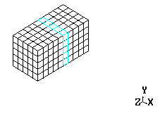
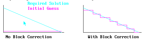
Library case 100 concerns the calculation of temperature distribution in a cube, with diagonally opposite corners held at different temperatures. It clearly shows the effects of the 1-D block corrections activated by ISOLX, ISOLY and ISOLZ. If these are removed, the convergence rate is much lower. It also shows the superior performance of the conjugate gradient solver, the effect becoming more marked as the grid is refined.

Library case 921 shows the use of user-defined block corrections. It concerns the prediction of flow and heat transfer in a closed cavity with a heated metal block. The air-space and metal block are treated as separate correction blocks.