 A 2D population
                   > transport of statistical quantities, (1)
                  /      following Kolmogorov's idea
                 /
                /
============>> /_________ > /
                /
                 /
                  /
                   > multi-fluid, ie discretized PDF     (3)
It will be further argued that the third, a natural extension of the
two-spike presumed-PDF approach, offers the best prospects.
The basic idea is that a fluid mixture, whether containing only one thermodynamic phase, or more than one phase (as in boiling, condensation or solid-fuel combustion), can be best treated as a "discretized population", as illustrated here.
                       __
      p =  proportion |  |                  ____
             of     ^ |  |         __      |    |___          __
            time    | |  |        |  |__ __|    |   |        |  |
      during which  | |  |        |  |  |  |    |   |__      |  |
      fluid has an  | |  |   _____|  |  |  |    |   |  |     |  |
      attribute value |  |  |     |  |  |  |    |   |  |     |  |
      within the      |  |__|     |  |  |  |    |   |  |     |  |
      abcsissa limits |__|__|_____|__|__|__|____|___|__|_____|__|
                                     ----------> a = attribute
The population can be described by:
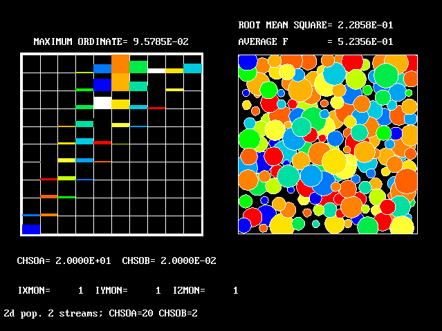
A 2-D population is created if two PDAs are selected, for example temperature and vertical- direction velocity.
An example of the graphical representation of a two- dimensional population is shown below.
The coloured proportion of each
box represent the mass fraction.
A 2D population
Three- and four-D populations can be envisaged; but they are harder to draw!
Material attributes which are not discretised (ie not selected to be PDAs) are called "continuously-varying attributes" (CVAs).
CVAs are treated as uniform in value (but different from each other) within each component of the population, and in each element of space-time.
PDAs are treated as uniform in value (but different from each other) only within each element of space-time.
The distinction between the two kinds of attribute is arbitrary; the analyst chooses as PDAs the attributes of which the fluctuation are most likely to be physically significant, for example the density when gravitation influences the flow.
If the selected PDA for a steam-water mixture is density and only two value bands are chosen, with the dividing value equal to the arithmetic-mean density of steam and water, the population is one- dimensional with two components.
It could be called a "2-fluid model"; and indeed the IPSA 2-phase- flow model, which has been in use for nearly two decades, is of this kind. An implication is that the steam and water temperatures, which are CVAs, have each only one value at a given point in the flow.
If it were then decided also to take account of the fluctuations of temperature, dividing the whole range into 10 equal intervals, temperature would have become the second PDA. The population would be 2-dimensional; and a "20-fluid" model would have resulted.
The task of numerical simulation of turbulence, with or without boiling, condensation, combustion, etc, thus becomes that of:
The said values are influenced by the physical processes of:-
These, and their interaction through the conservation laws of physics, are expressible by way of differential equations of well- known forms and properties.
So well-known are the equations that many widely-available computer programs are equipped to solve them. [ One such is the PHOENICS Shareware package.]
If, as usual, they are of the finite-volume kind, the programs compute the MFDFs and associated CVAs by solving a large number of inter-linked and non-linear balance equations by iterative techniques.
The most time- and attention-consuming part of the modelling exercise is then the formulation of the source-and-sink terms, which express (chiefly) how the distinct fluids interact with each other.
In the work to be reported below, the source-and-sink terms for the MFDFs have been derived from a physical hypothesis, based upon intuition rather that exact analysis.
            The "promiscuous Mendelian Hypothesis"
^ frequency in
| population         father                                  mother
|/          ______ /                                        /
|          |      |          promiscuous              ******
|        __|______|__ <------- coupling --------->   ********
|           | .. |                                   *| .. |*
|           |*  *|                                   *| -- |*
|           /-**--\      ____  Mendelian  ______      /-----\
|         /|//////| \   |      splitting        |   / |_____| \
|          |//////|     v                       v     /     \
|          |  ||  |    _     _    _    _    _    _  /_________\
|          |  ||  |   | |   | |  | |  | |  | |  | |   |  |  |
|          |__||__|   | |   | offspring |  | |  | |   |__|__|
--------------F--------O1----O2---O3---O4---O5---O6------M---------
                    fluid attribute -------------------------->
It may be deduced indirectly if a different attribute is chosen.
Moreover, there is nothing to prevent more-conventional means being employed.
For example, if the modelling study is focussed on chemical reaction rather than on hydrodynamics, the latter may be handled by the k- epsilon model, and mdot can be taken as proportional to k divided by epsilon.
The quantity mdot can be regarded as the micro-mixing rate. Something similar is used in earlier models such as those which presume the shape of the PDF or use the Monte-Carlo approach.