(2) Until May 2010, the material of the lecture was distributed between many .htm and .gif files. Their contents have now been collected into a single document for ease of distribution; and the opportunity has been taken to augment it by addition of previously omitted material, namely
This opportunity is exploited by the Multi-Fluid Model (MFM) of turbulence, which may be regarded as an extension and generalization of the "PDF-transport" model of Dopazo, O'Brien, Pope, et al. It is also the successor to, and generaliser of, numerous two- fluid models of the kind which were already envisaged by Reynolds and Prandtl.
MFM uses a conventional finite-volume method for computing the discretized PDFs, which may be one-, two- or multi-dimensional.
The lecture explains the nature and practical utility of MFM. Examples of its application to both chemically-inert and chemically-reactive flow phenomena are presented.
1. The task to be performed: computing the PDF
Computer simulation of many turbulent-flow phenomena, especially those influenced by body forces or chemical reactions, requires:
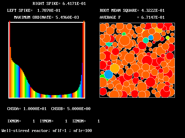
The following picture shows what is meant by a probability-density function.
The PDF is the curve on the left of the picture. The task is to calculate its shape.
On the right is a graphical reminder of the fact that a turbulent fluid consists of a random- seeming assembly of fluid fragments in various states.

The "spikes" on the left and right show that there are large amounts of extremely-cold and extremely-hot fluid.
The curve between them shows how much of the fluid is in the intermediate temperature ranges.
This information is needed for predicting, say:
Knowledge of the average temperature is of little or no use for these purposes.
This belief led to searches for labour-saving schemes, based upon
the presumptions that:
either
the PDF has a known, simple shape;
or
certain statistical properties of the PDF will suffice.
Both of these will be discussed in this section.
(a) The eddy-break-up model (EBU), (Spalding, 1971)
The eddy-break-up model for turbulent combustion represents the population distribution by two spikes, as shown:
              |
       mass   |   ^unburned
       fractions  |
       of the |   |
       two    |   |                ^burned
       gases  |   |                |
              |   |                |
              |   |                |
              |   |                |
              |___|________________|_____
                  0  reactedness-> 1
At any location, the gas
mixture is supposed to
comprise fully-burned and
fully-unburned gases.Their proportions vary with location in accordance with laws of convection, diffusion and source/sink interactions.
The latter represent the transformation of unburned to burned at a volumetric rate proportional to the local mean-flow shear rate.
In some variants, a chemical-kinetic rate-limitation was introduced.
The eddy-dissipation concept model for turbulent combustion also presumes a two-spike population distribution, represented as shown:
              |
       mass   |         ^mean mixture
       fractions        |
       of the |         |
       two    |         |
       gases  |         |
              |         |
              |         |    ^fine
              |         |    |structures
              |___|_____|____|_____|__
                  0  reactedness-> 1
At any location, the gas mixture is supposed to comprise mean mixture and "fine structures",
Their proportions vary with location in accordance with laws of convection, diffusion and source/sink interactions.
The latter involve mass transfer between the two gases at a volumetric rate proportional to the local mean-flow shear rate.
Chemical kinetics controls the rate of fine-structure reaction and so the mean-mixture reactedness.
The two-fluid model of turbulent combustion presumes a two-spike population distribution, represented as shown:
              |
       mass   |         ^slower fluid
       fractions        |
       of the |         |
       two    |         |
       gases  |         |
              |         |
              |         |    ^faster fluid
              |         |    |
              |___|_____|____|_____|__
                  0  reactedness-> 1
At any location, the gas mixture is supposed to comprise faster- and slower- moving gases.
Their speeds & proportions vary with location in accordance with laws of convection, diffusion and source/sink interactions.
The latter involve mass transfer between the two gases at a volumetric rate proportional to the local relative velocity.
Chemical kinetics controls the rate of chemical reaction within each gas, and so their individual reactednesses.
The latter tend to rise, and the former to fall, often with striking effects.
For example, hurricanes gather their destructive power from the fact that the upwardly moving moist-air fragments, as they rise to lower-pressure altitudes, shed much of their water content as rain.
The latent heat of condensation has the effect of increasing still further the disparity of density between the upward- and downward-moving fluids, the relevant motion of which is therefore maintained, despite the friction between them.
Two-fluid models of turbulence are well able to simulate such phenomena. For example, the present author showed [57] how PHOENICS could be used to calculate the variation with time of the upward- and downward-moving members of the "atmospheric population" as a consequence of the heating and cooling of the surface of the earth.
The following pictures represent what happens when a cool wind, moving from left to right, is heated as a consequence of contact with hot earth beneath it.


Not surprisingly, the upward-moving fluid has a higher temperature than the downward-moving fluid.
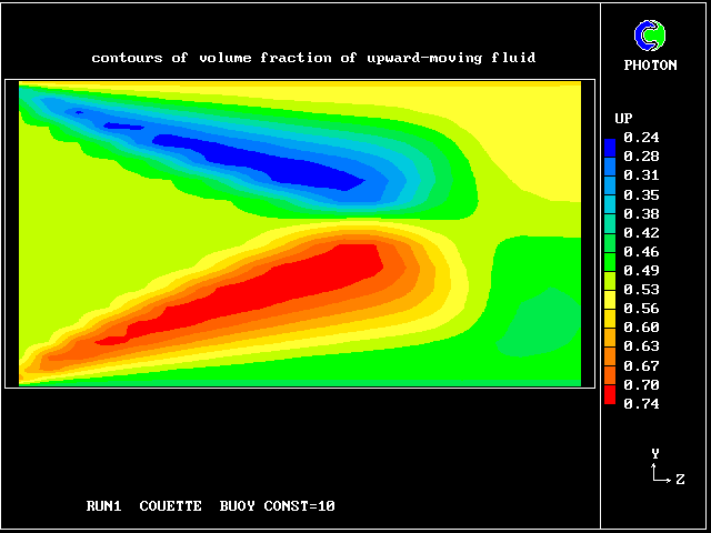
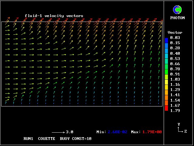
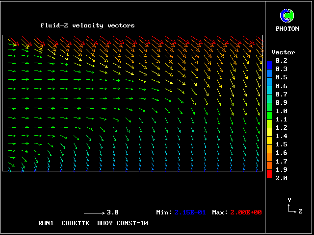
Some line-printer output from the PHOENICS library case W975 now follows; this concerns flow between a hot surface at rest and an upper cold moving surface. This is a Couette-flow idealization of an unstable atmosphere.
Each plot shows the variation with vertical distance of some properties of the two fluids, namely:
     ************************************************************

       Fig.1       1 =   V1   2 =   V2   3 =   W1   4 =   W2
         MINVAL= -1.871E-01 -1.871E-01  7.617E-13  7.617E-13
         MAXVAL=  1.875E-01  1.875E-01  2.000E+00  2.000E+00
     1.00 +....+....+....+...1+1..1+....+....+....+....+....4
          +          1 1 1 1        1                       +
          +   11 1 1                   1 1 1              443
          +111                               1 1 1 1 1 444 3+
          1                       4 4  4 4 4 4 4 4 4 4   331+
          +  444 4 4 4 4 4 4 4 4  3 3  3 3 3 3 3 3 3 3 33   2
          224    3 3 3 3 3 3 3                             2+
          +4 333 2 2 2 2 2                              222 +
          433              2 2                   2 2 2 2    +
          +                    2         2 2 2 2            +
     0.00 3....+....+....+....+...2+2..2+....+....+....+....+
          0    non-dimensional vertical height            1.0

     ************************************************************

       Fig.2       1 =   H1   2 =   H2
         MINVAL=  0.000E+00  0.000E+00
         MAXVAL=  1.000E+00  1.000E+00
     1.00 1....+....+....+....+....+....+....+....+....+....+
          +1                                                +
          2 1                                               +
          +2 111 1                                          +
          + 222    1 1 1 1 1 1 1  1 1  1 1 1 1 1            +
          +    2 2 2 2 2 2 2 2 2  2 2  2 2 2     1 1 1 111  +
          +                                  2 2 2 2 2 22 11+
          +                                              22 +
          +                                                21
          +                                                 +
     0.00 +....+....+....+....+....+....+....+....+....+....2
          0    non-dimensional vertical height            1.0

     ************************************************************

       Fig.3       1 = UP     2 = MDOT
         MINVAL=  0.000E+00 -2.038E-02
         MAXVAL=  1.000E+00  1.992E-02
     1.00 2....+....+....+....+....+....+....+....+....+....+
          +                                                 +
          +                                                 +
          +2                                                +
          + 2222 2 2 2 2 2 2 2 2       1 1 1 1 1 1 1 1 111111
          +                       2 2                       +
          111111 1 1 1 1 1 1 1 1       2 2 2 2 2 2 2 2 2222 +
          +                                                2+
          +                                                 +
          +                                                 +
     0.00 +....+....+....+....+....+....+....+....+....+....2
          0    non-dimensional vertical height            1.0

    ************************************************************
Despite the crudeness of the graphical representation, information
of physical interest can be derived. Thus, one may see from Fig.1
that the upward-rising fluid has the smaller horizontal velocity,
for the understandable reason that it comes from a lower-velocity
region.
Fig. 2 reveals that it is hotter than the downward-moving fluid, no doubt because it has received heat from the warmer regions, closer to the ground.
Fig. 3 shows that, according to this model, the volume fractions of the two fluids are not uniform. Thus there is more upward-moving fluid in the upper half (i.e.the right-hand half on the diagram) of the layer than in the lower. It is the inter-fluid mass-transfer rate (MDOT) which maintains the balance.
Before leaving this topic, it is worth remarking, to those to whom the two-fluid model is new, that this Couette-flow study can be regarded as a refinement of the idea which Ludwig Prandtl presented seventy years ago as the "mixing-length model". Prandtl had to make assumptions; whereas the two-model permits calculations. Thus, Prandtl had to assume that the differences of the vertical velocity were equal to the differences of the horizontal velocity, and that the volume fractions of the two fluids were equal.
As mentioned above, the two-fluid concept was inherent in the thinking of both Reynolds and Prandtl. To develop it further is to continue a distinguished tradition.
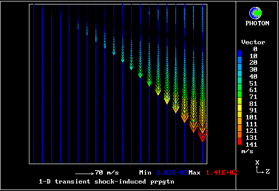
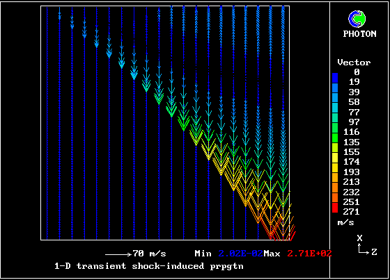
A shock wave passes down a vertical pipe containing a combustible gas which is burning slowly.
The wave accelerates the hot-gas fragments more than the cold ones, causing relative motion.
The relative motion causes increased entrainment and mixing, which leads to increases in the burning rate.
The increased rate increases the strength of the pressure wave.
The result is that the deflagration turns into a detonation.
The graphical plots show the development, the horizontal dimension being time.
The calculation was first performed in 1983. Its specification may be found in the PHOENICS Input-file library (case 893).
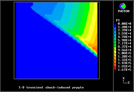
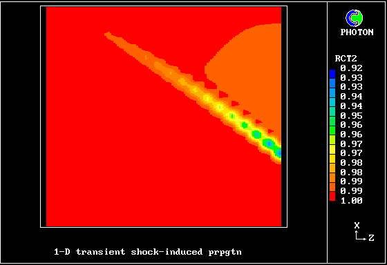
Contours of pressure (left) and reactedness of the hotter gas (right)
A steady stream of turbulent pre-mixed combustible gas flows into a parallel-walled duct. A flame, anchored by a centrally-placed flame- holder, spreads to the walls.
The parabolic-flow option of PHOENICS has been used for solving the four momentum equations, two energy equations and two mass- conservation equations.
The empirical constants employed concerned:-
The simulation featured in the Imperial College research of Jeremy Wu, 1987. It is now PHOENICS Input Library Case no W977. Agreement with experimental data, e.g.Williams, Hottel and Scurlock, is good.
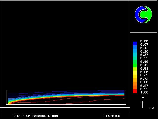
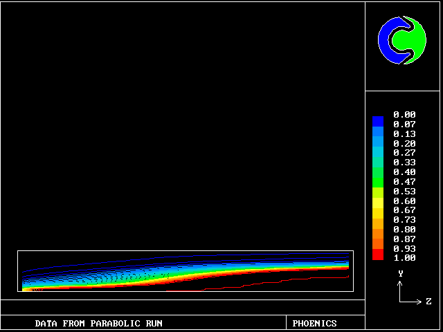
These contours differ from the previous ones, in that the cooler (slower-moving) fluid is the less reacted.
The two-fluid turbulence model is of use for other phenomena than combustion, and especially for those in which density differences interact with body forces.
Many examples arise in the atmosphere, lakes, rivers and oceans.
The two-fluid model, for example, can satisfactorily simulate the mixing-followed-by-unmixing behaviour when a salt-water layer, lying below fresh water, is heated for a short time.
            _________      _________      _________
           |         |    | * ** *  |    |         |
           |  fresh  |    |* *  * **|    |         |
           |         |    | * ** *  |    |         |
           |*********|    |* *  * **|    |*********|
           |* salty *|    | * ** *  |    |*********|
           |*********|    |* *  * **|    |*********|
            ---------      ---------      ---------
              start         later           later
                                            still
Mixing appears to take place soon after heating equalises the densities. But it is macro- not micro-mixing; so "unmixing" follows.
Experiments by Spalding and Stafford at Imperial College during 1979, in which the heating was effected by passing an electric current through the fluids, brought the mixing/unmixing phenomenon to light.
It was consideration of these experiments which prompted the development of the two-fluid model of turbulence, which has here been used to simulate it.
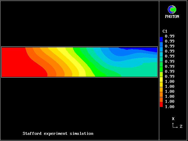
In this and the following pictures, which show contours computed by way of the two-fluid turbulence model:

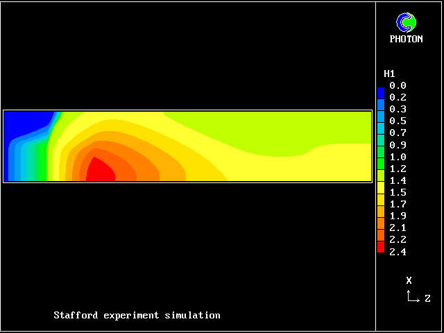
This picture shows how the temperature of the saline fluid first rises; it falls later, as heat is transferred to the fresh-water fluid.
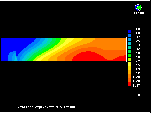
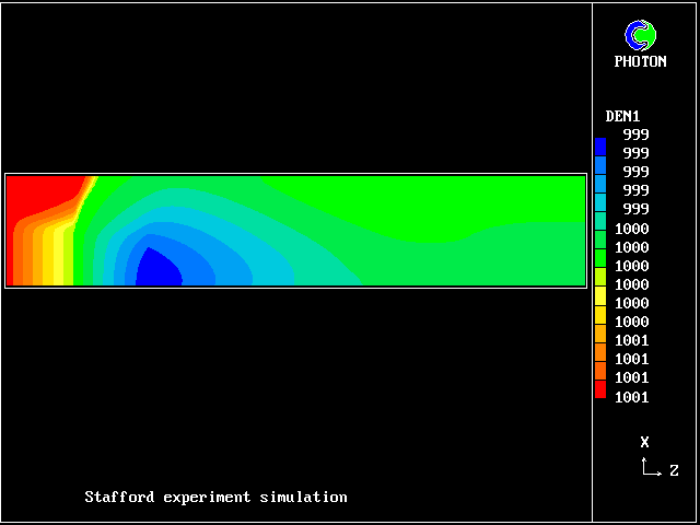
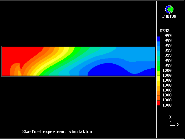
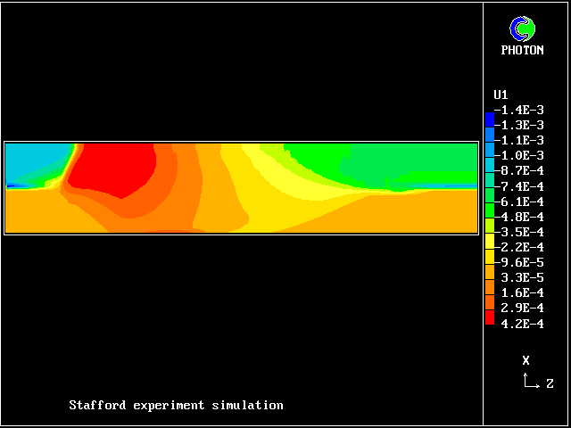

Here are the corresponding vertical-velocity contours of the fresh water
Later, cooling causes it to become negative again. Reminder: the horizontal dimension is time, increasing to the right.
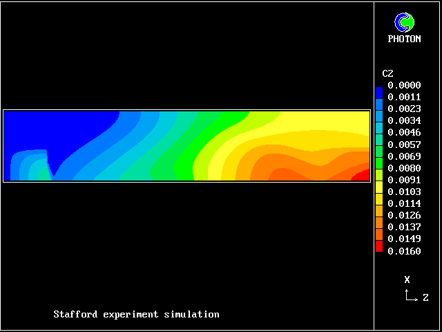
The simulation agrees qualitatively with the observations; but the "two-spike" representation of the fluid population is too crude for anything better.
Conventional turbulence models, for example k-epsilon, RNG, Reynolds-stress, etc cannot provide even qualitative agreement; for they lack the multi-fluids-in-relative-motion concept.
Phenomena of this kind are significant in many environmental phenomena, especially in the oceans.
The above-mentioned flames have concerned pre-mixed flames; but PDF shapes are often presumed for pre-mixed ones as well, the simplest presumption being the symmetrical-two-spike one.
       mass   |
       fraction
       of the |_0.5
       two    |         ^    ^
       gases  |         |    |
              |         |    |
              |         |    |
              |         |    |
              |___|_____|____|_______|_____
                  0 fuel fraction >  1
At any location, the gas
mixture is supposed to
comprise gases equally more
and less rich than the mean,
their deviations from the
mean being computed by way
of a transport equation for
the RMS fluctuations. Then the compositions of each gas are computed from the "mixed-is- burned" presumption.
Later authors have made more complex presumptions about the shape of the PDF, for example "clipped-Gaussian" or "beta-function".
These increase the amount of computation which is needed, sometimes very greatly; but it has not been demonstrated that the extra work is rewarded by improved realism of predictions.
As will be shown below, PDFs can vary greatly in shape from one part of a flame to another. Therefore, while two-spike models are useful because they promote physical insight with small computational cost, it can be argued that the more complex models increase obscurity rather than realism.
In any case, for non-pre-mixed turbulent flames, the PDF should be two- rather than one-dimensional, as will be explained below.
Currently popular turbulence models rely upon the presumption that all that needs to be known about a PDF is a few of its statistical properties.
AN Kolmogorov (1942) first proposed this; and he also postulated that two such properties, namely the energy and the frequency of the turbulence, obey differential equations of "transport" type, involving:
time-dependence, convection, diffusion, creation & destruction.
Later authors have employed different variables, eg:
(as just mentioned)
For fuller information about conventional turbulence modelling, see the article on turbulence modelling in the PHOENICS Encyclopaedia.
Nevertheless, methods of this (i.e.Kolmogorov-style) kind perform rather poorly for hydrodynamic phenomena when body forces (gravity, or centrifugal) are significant (as in Stafford's experiment); for they lack the "unmixing-because-of-body-forces" element.
Moreover they do not provide for calculation of the shapes of the PDFs, which are essential if chemical reaction is to be simulated.
Fortunately, despite popular belief, the Kolmogorov approach is not the only one which is available, as will be explained below.
Dopazo and O'Brien (1974) drew attention to the fact that differential transport equations could be formulated for the PDF itself. However, they did not provide numerical solutions.
When Pope (1980) did address the numerical-solution problem, he concluded that it was too difficult to solve with available methods and computers. He therefore introduced a Monte-Carlo approach to PDF transport, which has been adopted by the majority of later workers.
This approach undoubtedly reveals much about the phenomena to which it has been applied. Unfortunately its computational expense is still (rightly?) judged by practising engineers to be too great.
It appears also that Monte Carlo techniques cannot easily be used with some of the physical hypotheses which intuition suggests as being worthy of study in the present context.
Nevertheless, the pioneering work of these and other authors has influenced the recent developments of the multi-fluid approach.
                   > transport of statistical quantities, (1)
                  /      following Kolmogorov's idea
                 /
                /
============>> /_________ > Monte Carlo PDF                (2)
============>> /
                /
                 /
                  /
                   > multi-fluid, i.e. discretized PDF     (3)
It will be further argued that the third, a natural extension of the
two-spike presumed-PDF approach, offers the best prospects.
The basic idea is that a fluid mixture, whether containing only one thermodynamic phase, or more than one phase (as in boiling, condensation or solid-fuel combustion), can be best treated as a "discretized population", as illustrated here.
                       __
      p =  proportion |  |                  ____
             of     ^ |  |         __      |    |___          __
            time    | |  |        |  |__ __|    |   |        |  |
      during which  | |  |        |  |  |  |    |   |__      |  |
      fluid has an  | |  |   _____|  |  |  |    |   |  |     |  |
      attribute value |  |  |     |  |  |  |    |   |  |     |  |
      within the      |  |__|     |  |  |  |    |   |  |     |  |
      abcsissa limits |__|__|_____|__|__|__|____|___|__|_____|__|
                                     ----------> a = attribute
The population can be described by:
A 2-D population is created if two PDAs are selected, for example temperature and vertical- direction velocity.
An example of the graphical representation of a two- dimensional population is shown below.
The coloured proportion of each box represent the mass fraction.
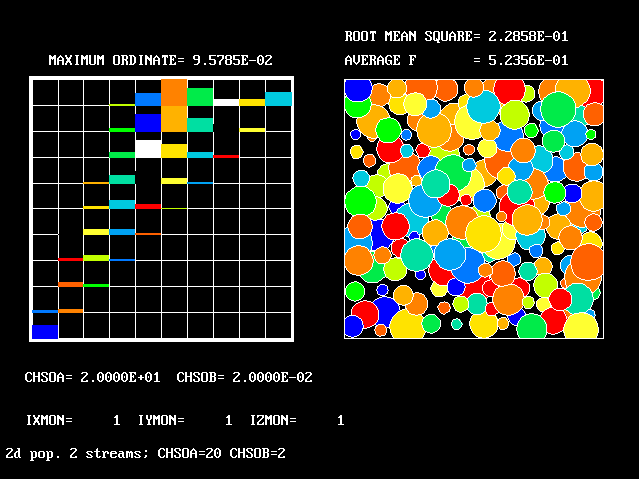
Three- and four-D populations can be envisaged; but they are harder to draw!
Material attributes which are not discretised (i.e.not selected to be PDAs) are called "continuously-varying attributes" (CVAs).
CVAs are treated as uniform in value (but different from each other) within each component of the population, and in each element of space-time.
PDAs are treated as uniform in value (but different from each other) only within each element of space-time.
The distinction between the two kinds of attribute is arbitrary; the analyst chooses as PDAs the attributes of which the fluctuation are most likely to be physically significant, for example the density when gravitation influences the flow.
If the selected PDA for a steam-water mixture is density and only two value bands are chosen, with the dividing value equal to the arithmetic-mean density of steam and water, the population is one- dimensional with two components.
It could be called a "2-fluid model"; and indeed the IPSA 2-phase- flow model, which has been in use for nearly two decades, is of this kind. An implication is that the steam and water temperatures, which are CVAs, have each only one value at a given point in the flow.
If it were then decided also to take account of the fluctuations of temperature, dividing the whole range into 10 equal intervals, temperature would have become the second PDA. The population would be 2-dimensional; and a "20-fluid" model would have resulted.
The task of numerical simulation of turbulence, with or without boiling, condensation, combustion, etc, thus becomes that of:
The said values are influenced by the physical processes of:-
These, and their interaction through the conservation laws of physics, are expressible by way of differential equations of well- known forms and properties.
So well-known are the equations that many widely-available computer programs are equipped to solve them. [ One such is the PHOENICS Shareware package.]
If, as usual, they are of the finite-volume kind, the programs compute the MFDFs and associated CVAs by solving a large number of inter-linked and non-linear balance equations by iterative techniques.
The most time- and attention-consuming part of the modelling exercise is then the formulation of the source-and-sink terms, which express (chiefly) how the distinct fluids interact with each other.
In the work to be reported below, the source-and-sink terms for the MFDFs have been derived from a physical hypothesis, based upon intuition rather that exact analysis.
            The "promiscuous Mendelian Hypothesis"
^ frequency in
| population         father                                  mother
|/          ______ /                                        /
|          |      |          promiscuous              ******
|        __|______|__ <------- coupling --------->   ********
|           | .. |                                   *| .. |*
|           |*  *|                                   *| -- |*
|           /-**--\      ____  Mendelian  ______      /-----\
|         /|//////| \   |      splitting        |   / |_____| \
|          |//////|     v                       v     /     \
|          |  ||  |    _     _    _    _    _    _  /_________\
|          |  ||  |   | |   | |  | |  | |  | |  | |   |  |  |
|          |__||__|   | |   | offspring |  | |  | |   |__|__|
--------------F--------O1----O2---O3---O4---O5---O6------M---------
                    fluid attribute -------------------------->
It may be deduced indirectly if a different attribute is chosen.
Moreover, there is nothing to prevent more-conventional means being employed.
For example, if the modelling study is focussed on chemical reaction rather than on hydrodynamics, the latter may be handled by the k- epsilon model, and mdot can be taken as proportional to k divided by epsilon.
The quantity mdot can be regarded as the micro-mixing rate. Something similar is used in earlier models such as those which presume the shape of the PDF or use the Monte-Carlo approach.
                                           |
At any location, the gas        mass   |   ^unburned
mixture is supposed to          fraction   |                 ^burned
comprise A (fully-unburned),    of the |   |  part-burned    |
D (fully-burned) and B and C    two    |   |     ^           |
part-burned, distributed        gases  |   |     |           |
in accordance with laws of             |   |     | part-burned
convection, diffusion and              |   |     |     ^     |
source/sink interactions.              |   |A    |B    |C    |D
                                       |___|_____|_____|_____|_____
The latter represent transformations       0  reactedness-> 1
A + D > B; A + D > C; B + D > C; A + C > B
at rates proportional to the local mean-flow shear rate.
Also C is both hot and unreacted enough to provide: C > D.
The first application of the 4-fluid model to a combustion process concerned the steady confined flame mentioned above.
The Prandtl mixing-length model of turbulence was employed for the hydrodynamics. This demonstrates, incidentally that one need not use the multi-fluid concept for all aspects of a phenomenon.
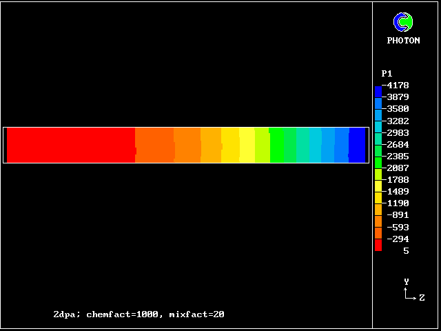
The following colour pictures show the results, which agree qualitatively and quantitatively with the Williams, Hottel, Scurlock data.
The flow is from the left, where the flame-holder is situated, to right. Only half the duct is shown, the symmetry axis being at the bottom of the picture.
Varying the reaction-rate constant (see the referenced paper) shows and explains how it comes about that the flame-spread angle is little influenced by its reduction until a sudden extinction occurs.
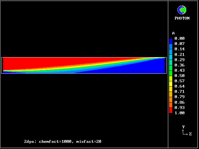
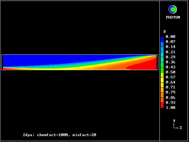
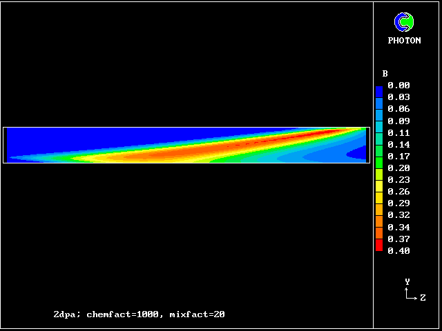
The comparatively low concentration of fluid C should be noted. It signifies that the reaction rate is high.
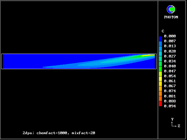
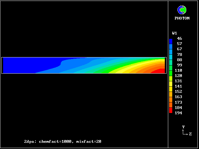
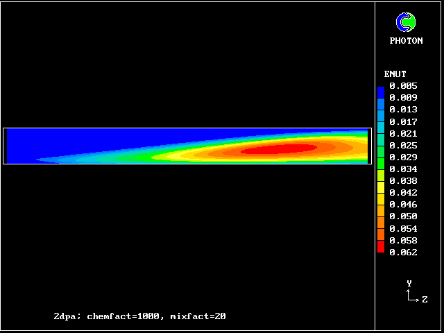
Its increase down the duct results from the increasing velocity gradient.
It concerns a duct filled with combustible gas which is ignited at the closed end. Flame spreads to the open end, causing a pressure rise in the duct.
The duct is partially blocked by transverse baffles in order to simulate the obstructions by solid objects which, by causing recirculations in their wakes, accelerate flames in confined spaces.
   wall__________________________________________________
 closed|       |      |      |      |      |      |     | open
    end| ignition                                         end
  axis |* --- - --- - --- - --- - --- - --- - --- - --- -
Comparisons with measurement, not provided here, show good agreement.
The 4-fluid model applied to unsteady flame propagation along a duct containing transverse baffles.

Note that the flame arrives last at a location not far from the ignition point. This is because the turbulence level is lowest there.
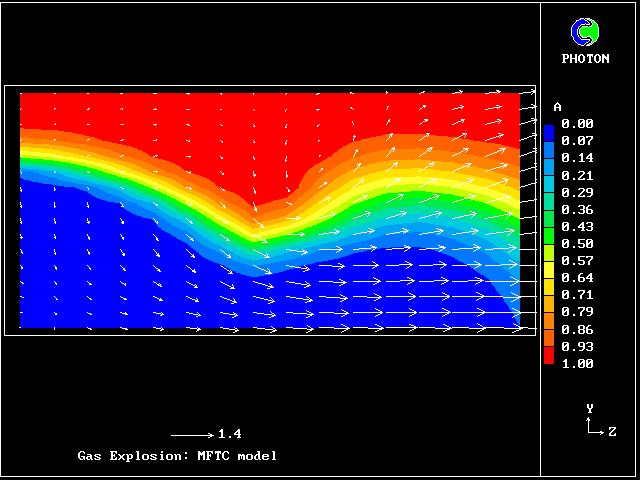
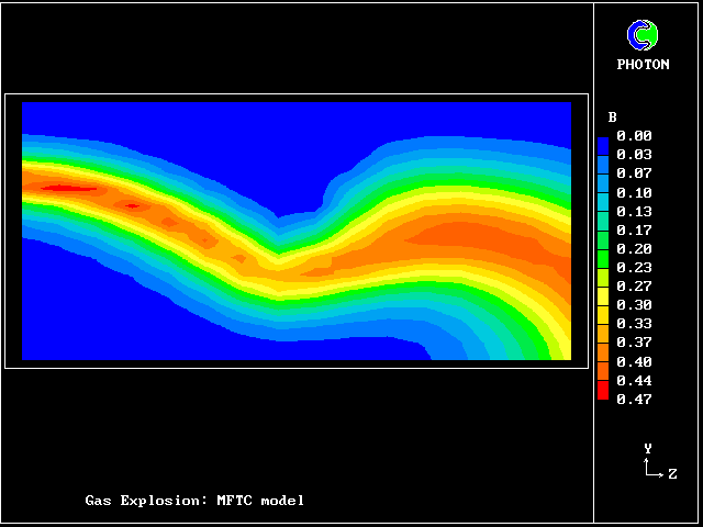

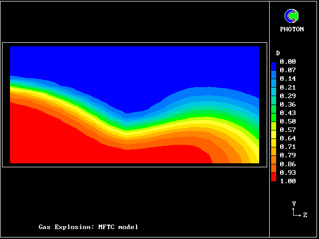
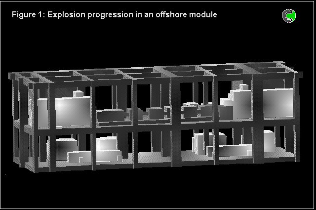
The 4-fluid model has also been used for numerous calculations concerned with full-scale models of off-shore oil platforms.
The problem is of course three-dimensional, transient, and complicated by a highly-obstructed space.
Comparisons were made with experiments, and with the predictions made by specialist computer codes having been subjected to "hindsight tuning".
The predictions based on the 4-fluid model were in at least as good agreement as those of the other codes; but there were uncertainties about the experimental conditions, as well as about the model constants.
The following pictures show some results.
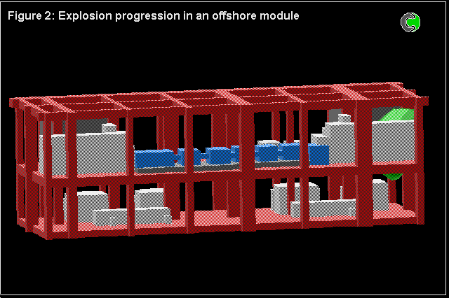
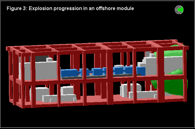
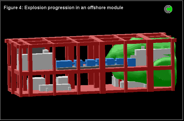
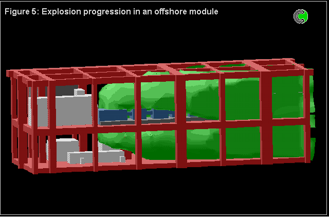
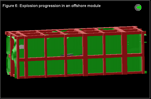
The four-fluid model increased the number of fluids by selecting an increasing number of fluid-defining values of a single attribute, namely the reactedness. It exemplified a one-dimensional fluid population.
However, multi-dimensional populations of fluids are generated when more than one attribute is used for fluid definition. This will now be illustrated, by way of the simplest example, namely a two- dimensional population. Once again, an example relevant to combustion will be chosen; specifically, values of fuel/oxidant ratio will be selected, as well as those of reactedness, so as characterise the population.
The following diagrammatic representation is copied from [40], where some of the main concepts of multi-fluid turbulence modelling are explained at greater length than has been possible here.
The 4-by-5 fluid-attribute grid, of which the ordinate can be regarded as reactedness and the abscissa as fuel-air ratio, represents a two-dimensional population.
     Fig.6 The 20-fluid population, of which only 14 fluids can exist
       _________________________________________
       |///////|///////|///////|       |       |
f - mfu|///////|///////|///////|  16   |  20   |  * mfu stands for
  ^    | inaccessible  |_______|_______|_______|    mass fraction
  |    | fluid states  |       |       |       |    of unburned
  |    |///////|///////|  11   |  15   |  19   |    fuel;
  |    |_______|_______|_______|_______|_______|  * fluid 1 is
  |    |///////|       |       |       |       |    fuel-free air;
       |///////|   6   |  10   |  14   |  18   |  * fluids 13-16
       |_______|_______|_______|_______|_______|    are stoichio-
       |       |       |       |       |       |    metric;
       |  1    |  5    |  9    |  13   |  17   |  * fluid 17 is the
       |_______|_______|_______|_______|_______|    fuel-rich entry
               --------> mixture fraction, f        stream.

************************************************************
Fluids 6, 11, 16 and 20 are supposed to contain no unburned fuel;
they thus represent completely-burned gases, of various fuel-air
ratios, which can react no further.
Fluids 5, 9, 13, 14, 17 and 18 contain finite amounts of free fuel; but they are regarded as being too cold to burn, like fluid B above.
Fluids 10, 15 and 19 both contain fuel and are hot enough to burn; it is therefore they which, like fluid C in the four-fluid model, carry out the chemical-reaction process.
Fluid 10 thus becomes transformed into 11, fluid 15 into 16, and fluid 19 into 20.
For example, fluid 5 can mix with fluid 19 so as to produce fluids 9, 10, 14 and 15, in proportions which the modeller is free to decide, on the basis of considerations which it would be distracting to discuss here.
A small stream of fluid 16 (stoichiometric combustion products) is supplied at the edge of the burner tube, to act as a lame holder.
  ************************************************************
    Fig. 7 Diagrammatic representation of the Bunsen-burner flame

   . /////////
   |  //flame/                | * PHOENICS is used to solve the
   .  ///////                 |   differential equations for 14
   |   /////     air at       |   fluid concentrations, as well as
   .   ////      rest,        |   for two velocities and pressure;
   |   ///       entrained    |
   /   ///       into         | * The parabolic (i.e.marching-
   |/  //        flame        |   integration) mode is used.
   .// //                     |
   | ////                     | * The Prandtl mixing-length model is
   .  //                      |   used for the hydrodynamics, and to
   ^^^^^| /                   |   supply local coupling-and-splitting
burner: |  / ignition         |   rates.
fuel-rich    source           |
gas jet |                     | * The grid is 20 (horizontal) and
                                  100 (vertical)

  ************************************************************
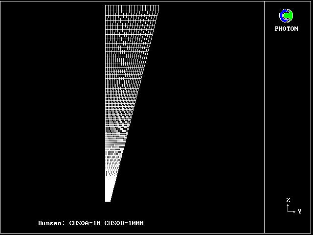
The Prandtl mixing- length model is used for the hydrodynamics.
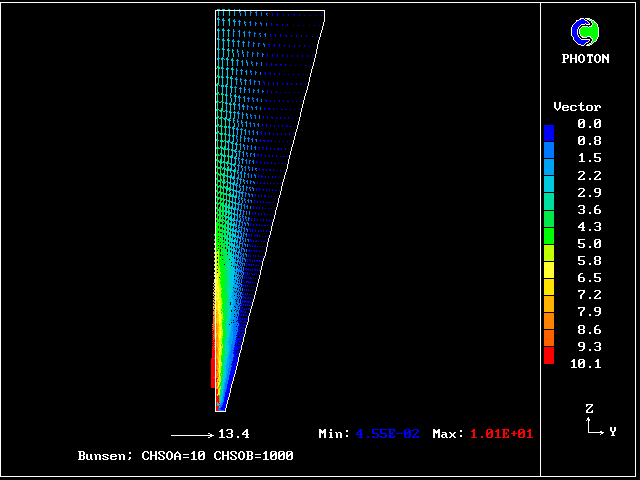
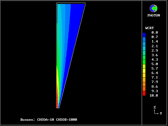
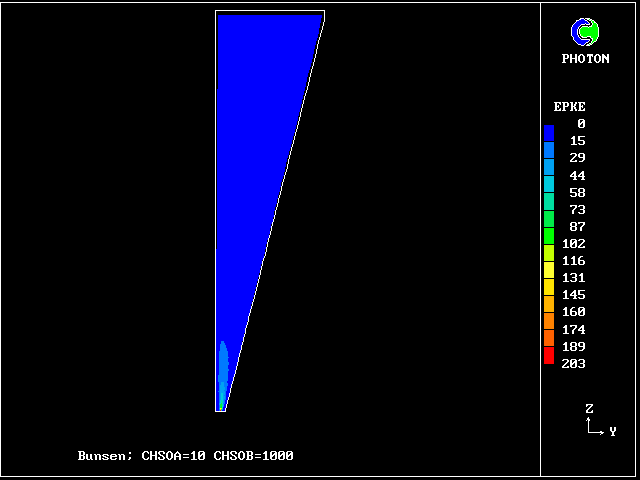
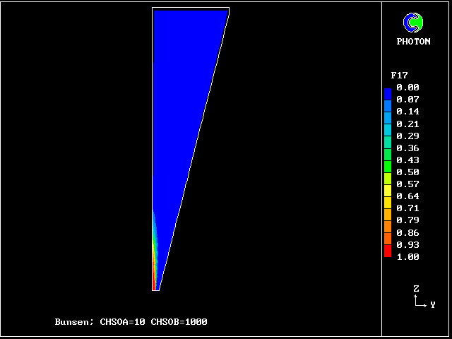
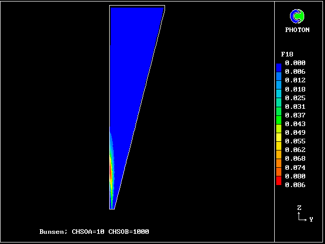
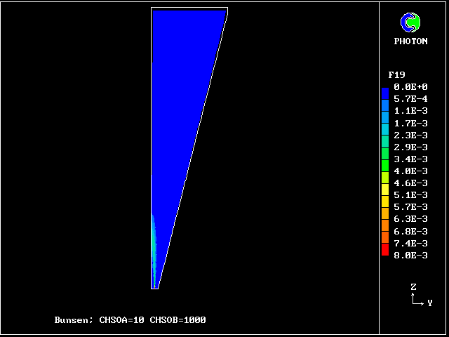


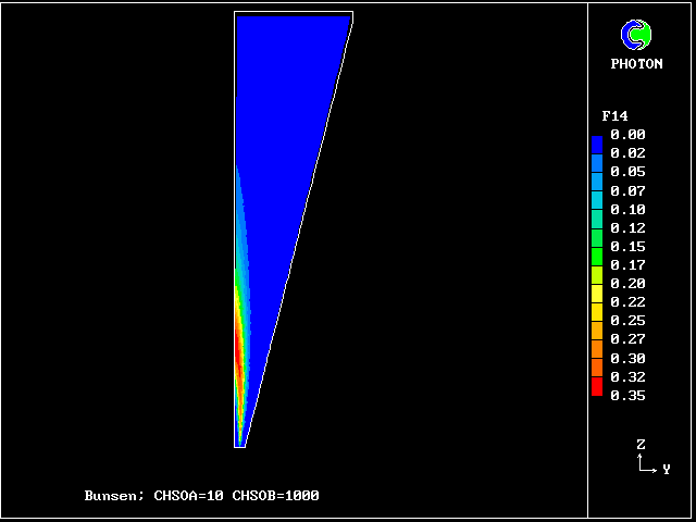
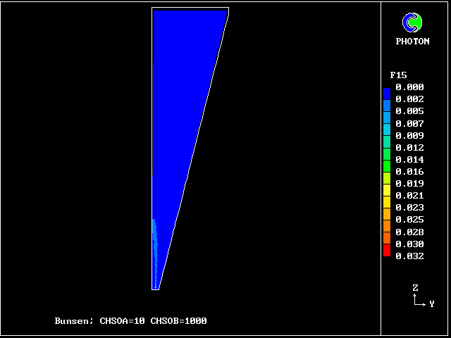
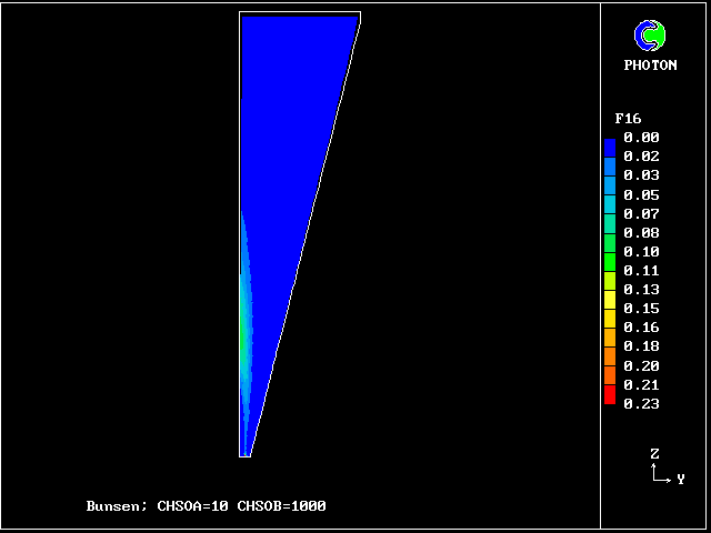

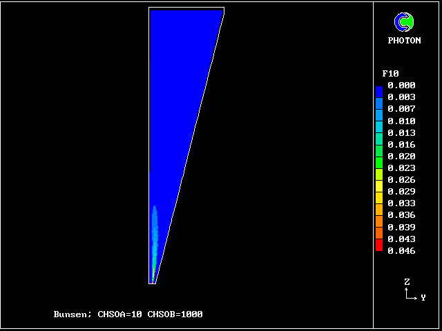
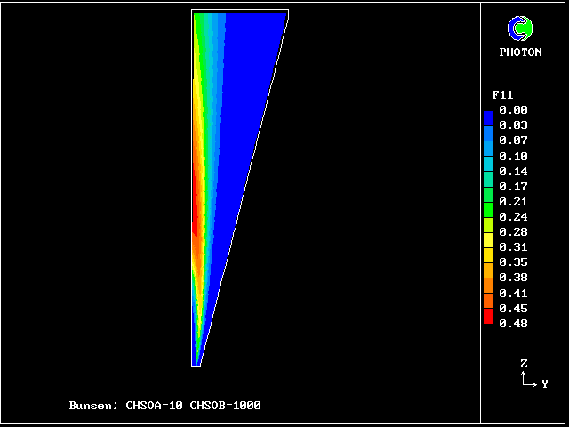
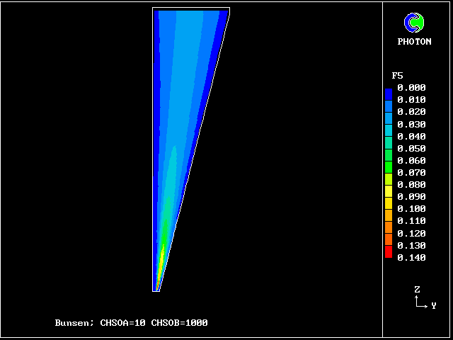
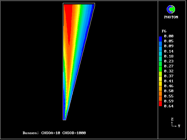
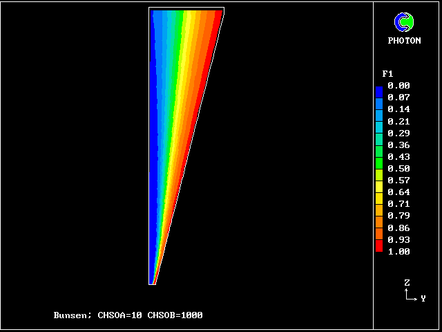
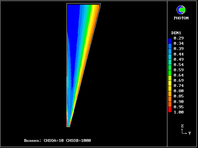
The plots of the concentration profiles of the fourteen distinct fluids are interesting; but it is hard to appreciate all their implications. Therefore another mode of representation has been devised by the author's colleague Liao Gan-Li.
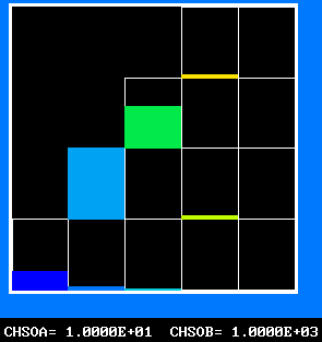
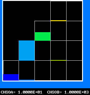
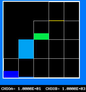
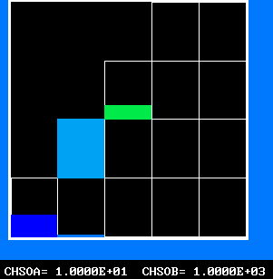
This shows the fluid population distributions directly, both as a conventional histogram and as a randomly distributed set of blobs. The following command lines create screen displays, when this file is viewed through polis. Otherwise the line-printer plots below may be inspected.
Colour pictures constitute a small selection of what can be deduced from the PHOENICS calculation.
The FDP for the location shown by IY (horizontal) and IZ (vertical)
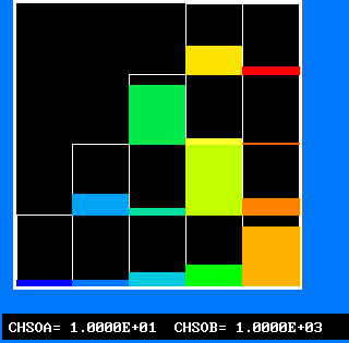
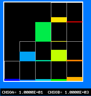
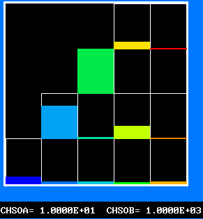


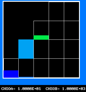
The following two line-printer plots, showing the profiles of concentrations of some of the fluids along the axis, provide some insight into how the fluids distribute themselves in the flame.
************************************************************
Fig.8 Axial profiles of the mass fractions of unburned fluids.
      Fluid 17 is fuel-rich supply gas; fluid 1 is air

  VARIABLE    1 = F17    2 = F13    3 = F9     4 = F5     5 = F1
    MINVAL=  6.654E-04  5.363E-13  2.382E-13  1.963E-13  4.988E-13
    MAXVAL=  9.988E-01  2.649E-02  4.516E-03  9.750E-04  2.688E-03

1.00 11111111111111.+....2223334444444..+....+....+55555
     +             111  2  3344433    4444   555555    +
     +               112  3 44   33     555554         +
     +                2113 4 22    33555      4444444  +
Fn's +               2  344   22   5533              444
     +              22 3441    2255   333              +
     +              2344  11   552      333            +
     +             244     1155  22        33333       +
     +           4443     55511    222         333333333
     +         4443 5555555   1111   222222            +
0.00 555555555555555+....+....+..11111111112222222222222
     --------- vertical distance above burner -------->
************************************************************
Fig.9 Axial profiles of the mass fractions of burned fluids
      Fluid 20 is fuel rich; fluid 16 is stoichiometric;
      fluid 10 is fuel-lean; fluid 6 is even leaner

  VARIABLE    1 = F20    2 = F16    3 = F10    4 = F6
    MINVAL=  1.246E-03  2.333E-12  9.055E-16  2.237E-13
    MAXVAL=  5.736E-02  3.175E-01  5.355E-04  1.271E-01

1.00 +....+....+....+....+...3333222222.+....+....+..444
     +                      33  33    2222        444  +
     +                     13  2 13       222  444     +
     +                    13  2   133       44422      +
Fn's +                   1 3 2     133   4444   22222  +
     +                  113 2       113444           222
     +                 113 2         44333             +
     +                113322      444  113333          +
     +               113322    4444     111133333      +
     +            1113332  44444           1111133333333
0.00 44444444444444444444444..+....+....+....+....111111
     --------- vertical distance above burner -------->
 ************************************************************
There are many important industrial flames, both desired as in furnaces and engines, and undesired as in oil-platform explosions, in which the fuel/oxidant ratio varies with position and time.
Means have hitherto been lacking for representing such phenomena in any but a single-fluid manner, with consequent inadequacy of realism.
The Bunsen-burner simulation just presented shows that a two- dimensional multi-fluid models can be created which will allow the fragmentariness of such flames to be taken more properly into account.
It seems certain that, when systematically exploited, this possibility will lead to better understanding and predictive capability.
For example, smoke and NOX production in gas-turbines should become easier to control.
                                                   _____|_____
 In the first example, it will be supposed        |     |     |
 that stream 1 is fully unreacted, that      1 ====>    |     |
 stream 2 is fully reacted, that 98 fluids        |  stirred  |
 of intermediate reactedness are created by       |  ///|/// 3===>
 micro-mixing and reaction (non-linearly          |  reactor  |
 dependent on reactedness) and that the      2 ====>          |
 outflowing stream 3 consists of 100 fluids       |___________|
 altogether, in to-be-computed proportions.
The flow is steady. Three cases will be shown, with mixing and reaction constants respectively = 10 & 10, 50 & 10, and 50 & 20.
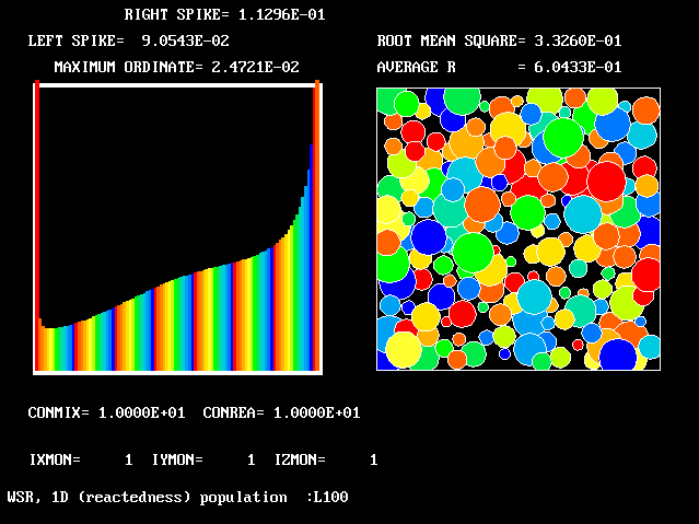
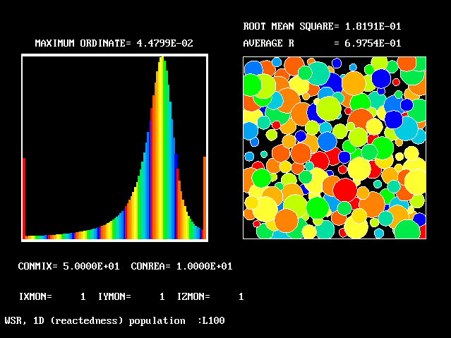
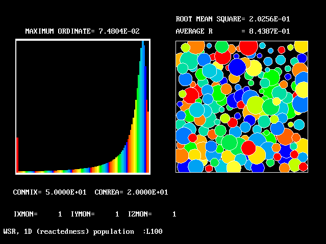
The necessary number of fluids may then become large; however, it is possible to determine the necessary number by grid-refinement studies.
Four results will be shown, for a well-stirred reactor in which the two entering streams are a fully-unreacted lean-mixture gas and a fully-reacted rich-mixture gas.
The population grids will be: 3 by 3 (too coarse) ; 5 by 5 (still too coarse) ; 7 by 7 (fairly good) ; 11 by 11 (more than fine enough). Inspection of the average reactedness reveals the solution quality.
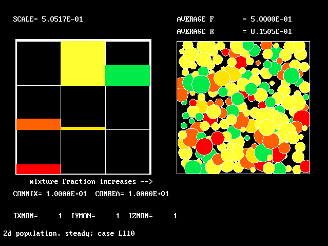
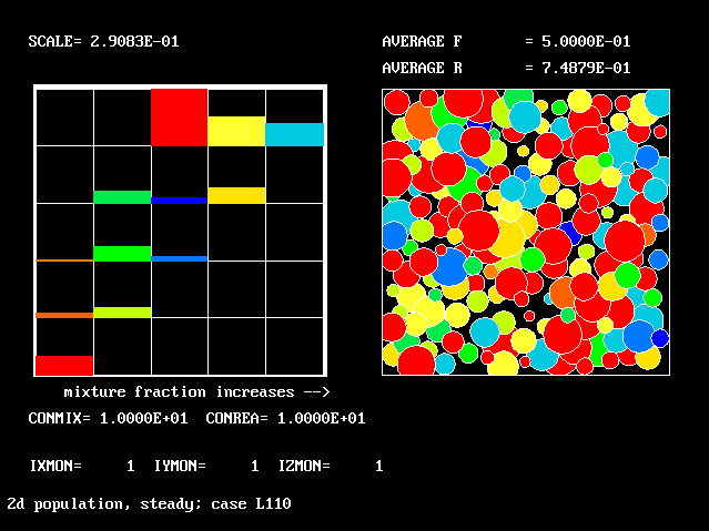
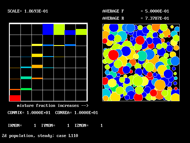
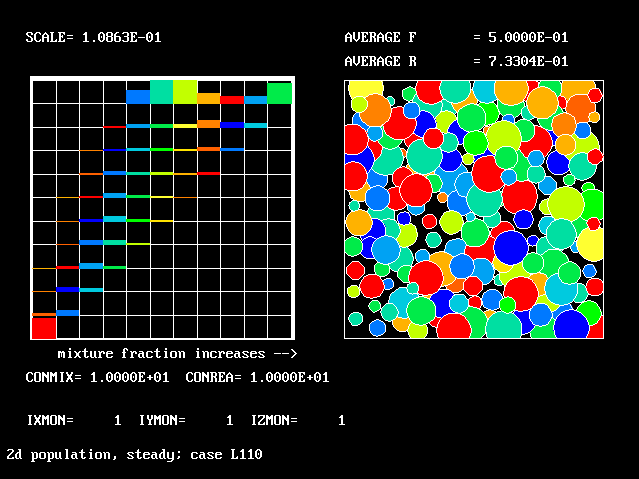
The shapes of the PDFs for the pre-mixed case vary with the values of the mixing and reaction constants (and of other parameters too, of which time-shortage precludes mention). They are "clipped-Gaussian" or "beta-function" only by (rare) chance.
The use of the 2D population for the non-pre-mixed reactor goes beyond what any "presumed-PDF" practitioner has ever dared (or should dare) to presume. Once again, the population distribution varies greatly with the defining parameters.
Such calculations take very little time; but pondering their significance needs much more. More "ponderers" are needed.
The cases shown are standard items of the PHOENICS input library; so any interested researcher can access and exercise them.
The productivity of the reactor depends greatly on the effectiveness of the micro-mixing; but until the arrival of the Multi-Fluid Model, there was no practicable way of predicting this.
The prediction problem is complicated by the facts that the geometry is three-dimensional; and unsteady analysis is needed in order to represent properly the effects of the stirring paddle and of the rotation-impeding fixed baffles.
In the following extract from a recent study, PHOENICS has been used for the simulating such a reactor; and the use of the multi-fluid model has revealed the importance of being able to simulate the micro-mixing process.
The reactor is one for which the US Dow Corporation has reported experimental data (only hydrodynamic data, alas!) which have been used in "benchmark studies".
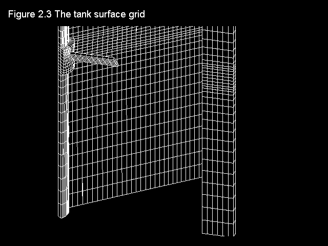
The geometry and computational domain are shown below.
The impeller speed is 500 rpm, the dynamic laminar viscosity is 1.0cP and the water density is 1000 kg/m
The computational grid is divided into two parts, namely an inner part which rotates at the same speed as the impeller, and an outer part which is at rest.

The total number of cells is 31365 (45 vertical, 41 radial and 17 circumferential).
                                           __________|.|__________
The sketch illustrates the apparatus and  |          |||          |
the initial state of the two liquids.     | upper    |.|          |
                                          | liquid   |||          |
They are both at rest, and are separated  |          |.|  acid    |
by a horizontal interface                 |..........|||..........|
                                          | lower    |.| alkali   |
The paddle is supposed to be suddenly set | liquid   |||          |
in motion.                                |       ---------       |
                                          |paddle /////////       |
The computational task is to predict both |           .           |
the MACRO-mixing, represented by the      ------------|------------
subsequent distributions of time-average              .< axis of
pressure, velocity and concentration, and                rotation
the MICRO-mixing, i.e.the extent to which the   The paddle-stirred
two liquids are mixed together at any point.       reactor
There is no need, simply because MFM is available, to refrain entirely from using conventional models.
In the present study, therefore, the k-epsilon model was used as the source of the length-scale, effective-viscosity and micro-mixing information.
This allowed the power of the MFM to be concentrated on the process which it alone can simulate, namely micro-mixing and the subsequent chemical reaction.
An eleven-fluid model was employed, with mass-fraction of material from the top half of the reactor (i.e. the acid) as the population- distinguishing attribute.
This was probably not sufficient to permit achievement of grid- independent of solutions. However, one of the merits of MFM is that population-grid-refinement studies are easily performed.
The simulation procedure therefore generates a very large volume of data, of which only a tiny fraction can be presented here.
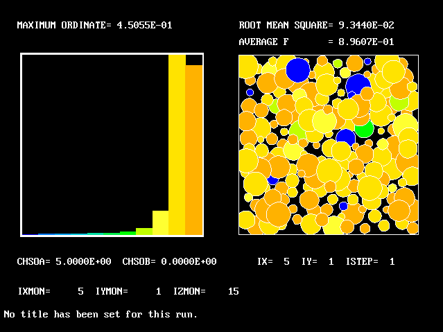
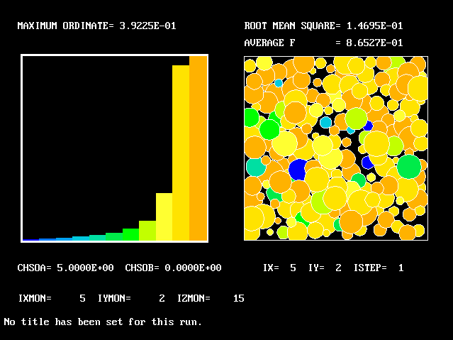
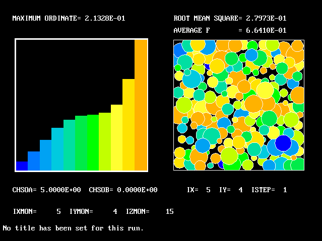
What will first be shown is a series of PDFs. They all pertain to:
Specifically, FPDs will be shown for six radial locations, starting near the axis and moving outward to about one third of the radius.

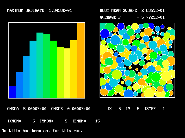
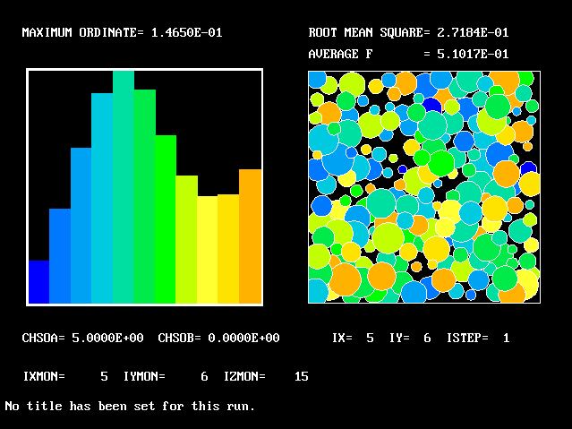
The acid and the alkali are supposed to react chemically in accordance with the classic prescription:
acid + base -> salt + water
Of course, no chemical reaction can occur in the unmixed fluids, which (to use the parent-offspring analogy) are the Adam and Eve of the whole population. It is only their descendants, with both acid and alkali "in their blood", who can produce any salt.
This is why the prediction of the yield of salt necessitates knowledge of the concentrations of the offspring fluids.
The next picture shows the salt concentrations after 10 paddle rotations which the multi-fluid model has predicted.
These concentrations are the averages for all eleven fluids.
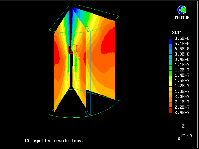
They are greatest in the region which has been most vigorously stirred by the paddle, which tends to thrust fluid downwards and outwards.
If no account is taken of the existence of the fluctuations, as is perforce the usual case, only the mean value of the acid/base ratio is available.
If the salt-concentration distribution is calculated from this, as the next picture will show, the values will be different from before.
Indeed it can be expected that they will be larger, because the implication of using a single-fluid model (which is what neglect of fluctuations amounts to) is that micro-mixing is perfect.
This is indeed what is revealed by the calculations.
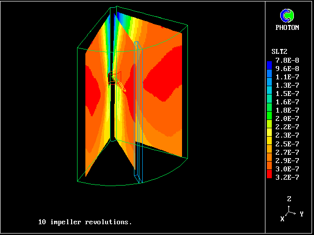
They are larger than the multi- fluid values, because micro- mixing is presumed (wrongly) to be perfect.
The following conclusions appear to be justified by the studies conducted so far:-
Guessing this is dangerous; but MFM can compute it.
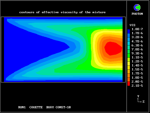
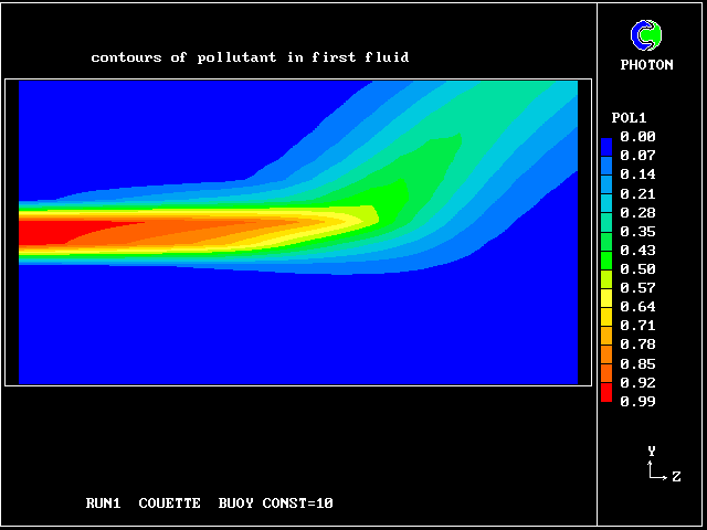
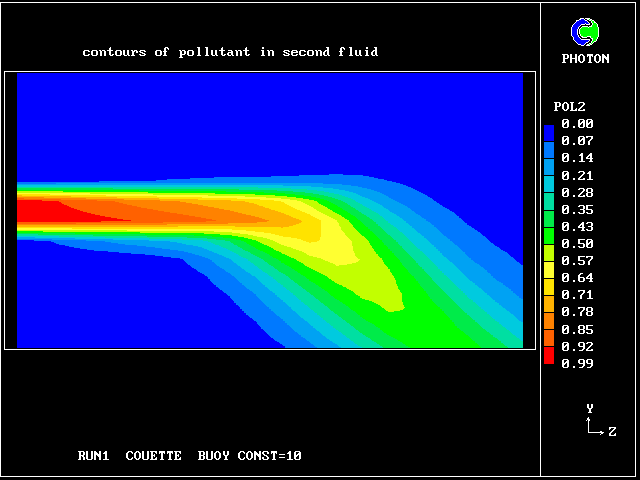
The following pictures result from exercising another case from the PHOENICS library. The smoke-kinetics formula is highly idealised, so as not to obscure the main message: MFM can be used in practice now.
The pictures show the distributions of smoke concentrations at the outlet cross-section based on:-
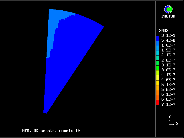


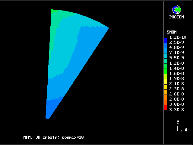
Computer times are, in any case, not very large, that for 20 fluids being only three times that for a single fluid.
However, when 100 fluids (say) do prove to be necessary on grounds of accuracy, there are many available means of reducing the computer times.
For example, there is no need to employ the same number in all parts of the field; instead, the number can be varied according to the local behaviour of the solution.
Once, indeed, that it is recognised that MFM entails nothing more than discretizing dependent variables in the same way as is routine for independent ones (space and time), the well-known techniques of grid-adaptation become available.
Axial-flow compressors and turbines, as used in aircraft propulsion and in ground- (or sea-) level power production, are characterised by the rapid passing of one blade row behind another.
The slower-moving boundary-layer fluid from the upstream row becomes a "wake" of slower-moving fluid fragments, which are distributed across the entrance plane of the downstream row.
The turbulent mixture which passes from row to row through a turbo- machine is therefore best represented as a population of fluids, with (say) axial velocity as their distinguishing characteristic.
MFM, provides a practicable means of calculating the population distribution and its influence on the mean flow, i.e.the "losses", which Kolmogorov-type models are failing to predict correctly.
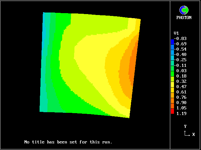
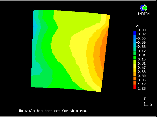
There follow two pictures which show how the time-mean velocity distribution of a blade row differs according to whether a two- fluid or (as is customary) a single-fluid model is presumed.
The differences are qualitatively similar; but the small quantitative differences are what count when blade-row losses are to be computed.
If two-fluid calculations can already provide meaningful guidance to turbo-machinery designers, much more can be expected from the full MFM treatment.
Unfortunately, most turbo-machinery researchers still follow each other down the approach-1 tunnel, with no light at the end! To switch some effort to MFM would appear timely.
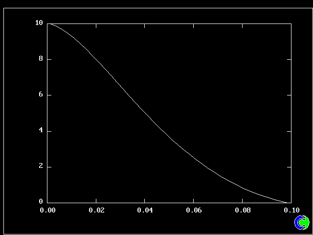
Such layers have been much studied, both experimentally (e.g. by Reichardt, 1942) and theoretically (e.g. by Tollmien, 1926). It is known that the profile approximately fits the formula:
W' = [ 5 * Y' ** 2 - 2 * Y' ** 5 ] / 3
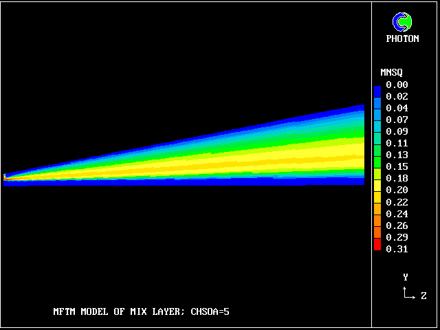
MNSQ is defined as the local root-mean-square velocity fluctuation.
Its cross-stream width increased from nearly zero to 0.725 m at a distance of 3.12 m from the start.
The flow-direction velocity of the entering stream, designated as fluid 1, was 10 m/s; the reservoir fluid, designated as fluid 40, had a flow-direction velocity of zero.
These fluids entered the wedge-shaped computational domain, through its two inclined boundary surface, at the rates necessary to ensure conservation of momentum, total mass, and the satisfaction of the transport equations of all 40 fluids. They were outcomes of the calculation rather than bondary conditions.
The calculations were performed by the PHOENICS code, working in parabolic mode. The calculation took 642 seconds on a Pentium 200 PC.
So one does not have to wait long for results, some of which now follow. [The date may be noteworthy; it is that of the first- ever hydrodynamic-flow calculation based on MFM]
First, some velocity-vector concentration-contour plots will be shown. These will be followed by some computed PDFs.
The above-mentioned results are those of the 1996 calculation. Nowadays such calculations are routine, there being a mixing-layer example in the latest PHOENICS Input-File library.
The cross-stream profiles shown below come from the library case.
The velocity vectors are as expected.
The grid is an expanding one, with 40 intervals across and 100 along the layer.
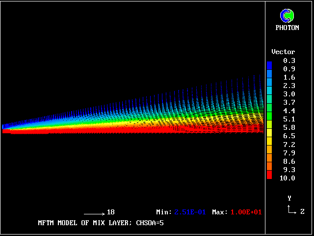
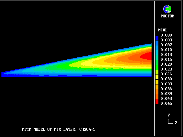

Agreement with experiment is good.
The following picture shows contours of the average concentration (for all 40 fluids) of material emanating from the upper stream.
It is just as a conventional turbulence model (e.g. mixing-length or k-epsilon) would reveal; but no transport equations for statistical quantities are being solved.
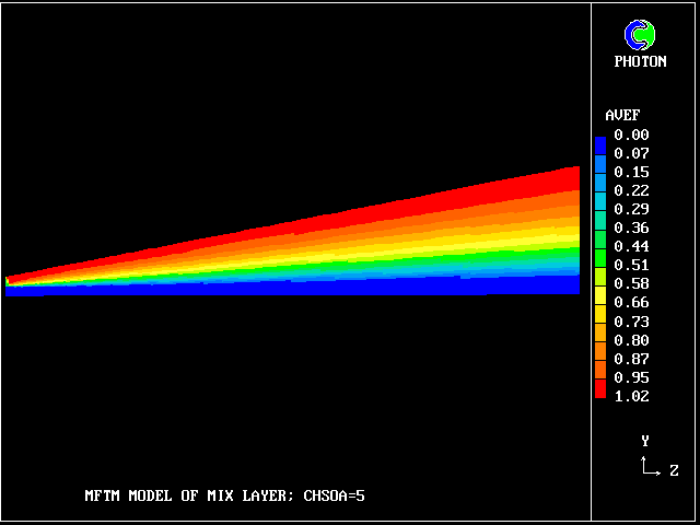
But how much upper-stream fluid (fluid 40) remains in its pure state? Only this.
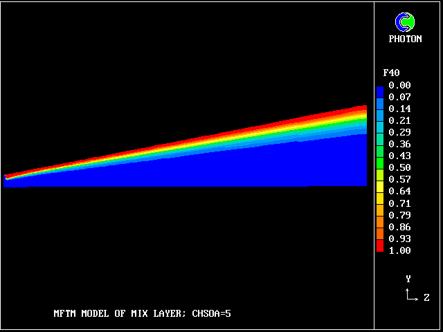
Where has the rest gone?
What about pure lower-stream fluid?
It also occupies very little space.
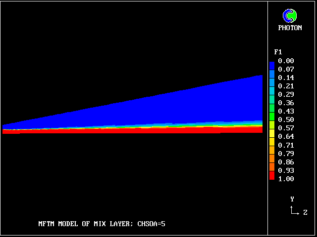
So what lies in between? 38 other fluids, variously intermingled.
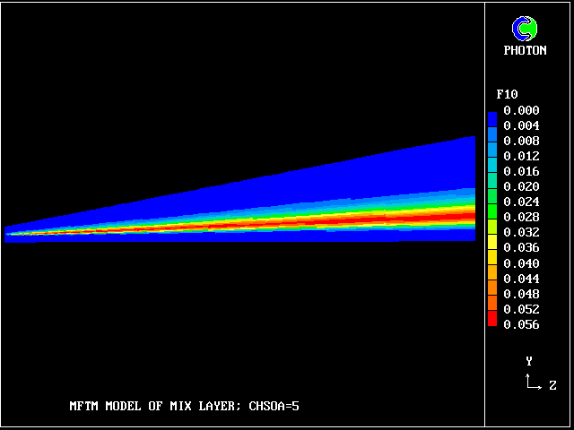
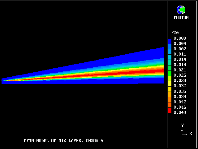
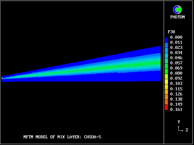
The results can be processed and displayed in many different ways.
Particularly relevant to the theme of the present paper are the discretized probability-density functions (PDFs), which may also be called:
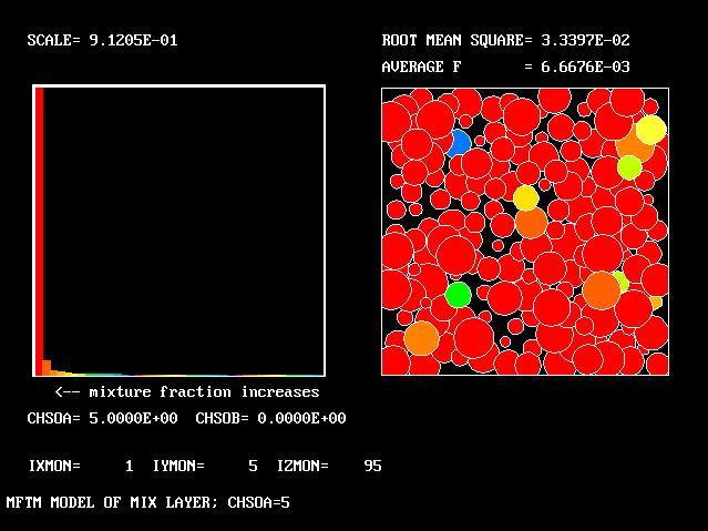
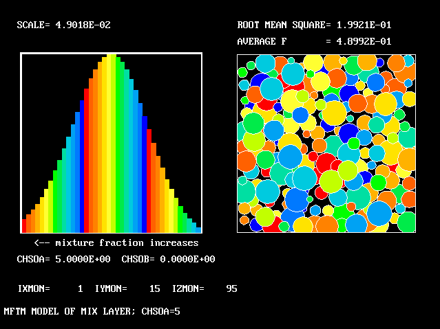
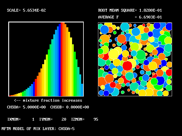
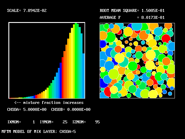
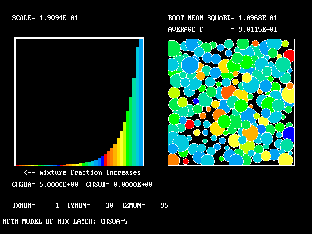
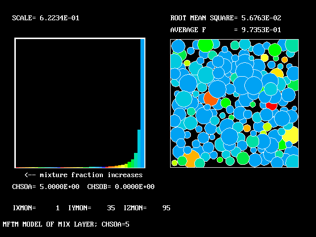
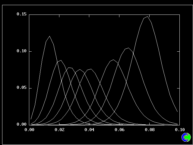
The PDFs are on the left in the next pictures.
The displays on the right are reminders of how the population of fluids might be distributed in a single computational cell, namely at random.
All the PDFs to be shown relate to a downstream section of the mixing layer, where the profiles are fully developed.
The first relates to a location near the lower (higher-velocity) edge of the layer.
The population consists almost entirely of higher-velocity fluid

All that has been used so far is the root-mean-square velocity fluctuation, as an input to the formulae for:-
As expected, a self-similar distribution is found.
The value along the "spine" of the layer is approxinately 20 % which is in order-of-magnitude agreement with experimental data.
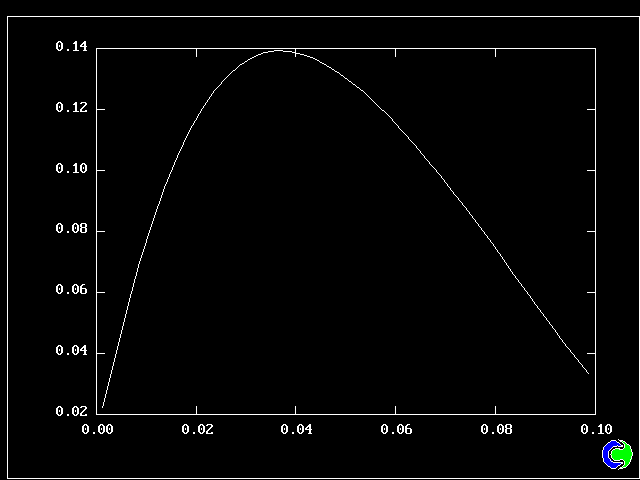
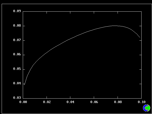

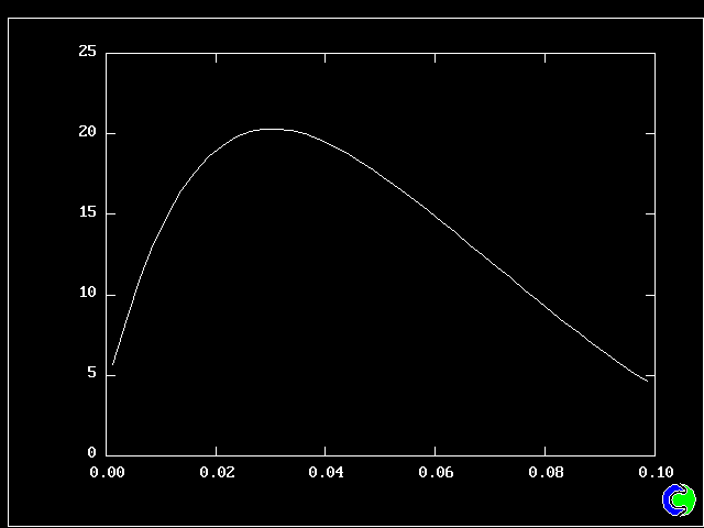
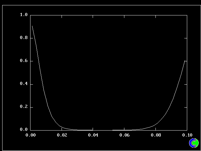
The width is here defined as the distance across the layer between the points where the mean velocity is 0.1 and 0.9 times the maximum velocity. With this definition. the rate of-spread ratio is found to be: 0.153 .
Other numerical results of interest are, for the fully-developed region, the following dimensionles numbers:
8.3 Comparison with experimental data
(a) Rate of spread, etc
An experimental investigations by Reichardt (1942) has shown that:-
Passive-scalar profiles are not exactly the same as longitudinal- velocity profiles in plane mixing layers, but have the less-curved shape which corresponds to an effective Prandtl number of less than 1.0.
Nevertheless, it is gratifying to note that the shapes of the PDFs reported by Batt are in qualitative accordance with those presented above, varying from near-symmetry in the centre of the layer to marked "lopsidedness" near the edges of the layer.
It may also be of interest to note that Fueyo et al (1995) reported a numerical study of the mixing layer by means of a Monte-Carlo- based method. Their reported PDFs were similar to those of the present paper; but the computer time, with 600 computational cells compared with the present 4000, was 45 minutes on a Convex C220 .
In particular, the multi-fluid model predicts the overall flow characteristics as well as a conventional model; and, because it computes the PDFs, as a conventional model cannot, it provides much more detailed insight into (what may be) the physics of the flow.
Nevertheless, no investigation has yet been made as to whether the constants which were found appropriate for the mixing layer will serve also for other flow situations.
Further, it needs to be established whether the discretization was adequately fine, in respect of the finenesses of the both the geometric and population grids. The PHOENICS library case facilitates this.
9.1 Concluding remarks about the nature of MFM
Contents of section 9.1
Such efforts as have been exerted (see ICOMP, 1994), apart from the author's own, have adopted the Monte Carlo method; this, however, has heavy computational requirements, and makes unusual intellectual demands. For these reasons, it is little used.
MFM is computationally less expensive than Monte Carlo; it employs computational methods which are familiar to all CFD practitioners; and it has advantages (such as grid-refinement and coarsening) of its own.
Now is therefore the time to consider what opportunities exist for its further development, and what research activities are needed so as to allow these opportunitires to be exploited.
(c) Especially promising practical applications
In addition to those applications mentioned in this lecture, e.g. to
turbo-machinery, paddle-stirred reactors and gas-turbine combustors,
there are several application areas for which MFM is especially
promising. They include:-
Already it has been applied (Svensson, 1996) to simulation of ground-water flow beneath Scandinavia since the last Ice Age!
9.2 Mathematical and computational tasks
Contents of section 9.2
(a) Population-grid refinement
It is necessary to establish, for a much wider range of problems
than has been investigated so far, that refining the population grid
(i.e.increasing the number of fluids) does indeed always lead to a
unique solution, and then to establish how the accuracy of solution
depends upon the grid fineness.
This needs to be done for many one- two- and (at least a few) three- dimensional population grids, before the basic ideas and solution algorithms will be widely accepted as sound.
There is little doubt that they ARE sound; but it is also important to gather information about how the fineness necessary for (say) 5% accuracy depends upon the process in question, and about local conditions.
Such information will assist automatic-grid-adaptation studies.
When the micro-mixing constant becomes very large, the behaviour of the population of fluids must reduce to that of a single fluid, of which the PDA values vary from place to place.
It needs to be checked that the system of equations does indeed exhibit this behaviour, and that the right values are calculated for the fluid concentrations.
A prudent and insightful investigator will wish to devise other tests of a self-consistency or conservativeness character before he wholly trusts his mathematical apparatus; and he will apply these tests in the largest possible variety of conditions.
(c) Non-uniform, unstructured, and self-adaptive grids
So far, the author has used only uniform and structured grids, which
have remained the same throughout the computation; yet there are
obvious advantages to be gained by relaxing these restrictions.
Thus, it may be convenient to define the attribute to be discretised as the ratio of the current temperature to the maximum temperature in the field, which temperature may change throughout the period of the calculation. Such a grid would have to be self-adaptive.
Another kind of self-adaptive grid would change its uniformity as the calculation proceeded, so as to capture with maximum accuracy the shape of the fluid-population distribution.
Yet another would insert new subdivisions of the PDA in regions of steep variation, and remove them from regions of less interest.
In summary, all the ingenious devices which specialists have invented for the better representation of variations in geometric space are likely to have their population-grid counterparts.
Fortunately, numerous methods of load-reduction exist, including:
There are however many practical applications in which the CVAs will
be of greater importance. These include:-
Three kinds of comparisons should be distinguished, namely:
(d) Computational improvements
Although the computer-time burden is not yet great, it may become
less tolerable when fine-grid three-dimensional transient simulations
with complex chemical kinetics have to be undertaken.
It will also be necessary to devise optimal overall discretization
strategies; for certainly it is not optimal to employ an extremely
fine geometric grid when the population grid is too coarse to
represent adequately the fragmentariness of the flow.
(e) Attention to the continuously-varying attributes (CVAs)
Although CVAs have made their appearance in the examples presented
above, namely as salt and smoke concentrations, they have played
only a subordinate role.
When it is recognised that the PDA/CVA distinction is arbitrary, and
that rational principles of selection are needed, it can be seen
that much experience needs first to be gained.
9.3 Tests of realism
Contents of section 9.3
(a) Comparisons with experiment
In order to establish the predictive capabilities of MFM now and in
the future, it is of course necessary to make comparisons with
experimental data.
(b) Comparison with the results of direct numerical simulation
(DNS)
One more comparison type should be mentioned, namely:
4. that with the results of direct numerical simulations.
DNS has become an increasingly popular tool of turbulence researchers; and indeed it is an excellent, albeit expensive, means of investigating what truly happens in a turbulent flow.
Until now, the outputs of DNS studies have been mainly used for comparison with the predictions of conventional (i.e.Kolmogorov-type) turbulence models; yet complete PDFs can equally-well be produced.
When serious research into MFM begins, one of its important elements will certainly involve the use of DNS for distinguishing between alternative micro-mixing concepts, and for establishing the appropriate constants.
(c) The order of events
Were there no urgency about solving the practical problems of
engineering and the environment, a rational research program would
probably concern itself first of all with kinds (2) and (4), in
order to establish a convincing prima faci.e.case for MFM.
Then experiments would be conducted systematically so as to permit kind-(3) comparisons, leading perhaps to improvements in particular model features.
Finally, comparisons of kind (1) would be made, whereafter, if the agreement proved satisfactory, industrial use of MFM would begin.
However, perhaps fortunately, there IS much urgency; for the models which are currently used for predicting turbulent chemical reaction in particular are far from satisfactory.
It therefore seems reasonable that some comparisons of kind (1), ie between MFM predictions and industrially-important phenomena, should begin in the near future.
9.4 Conceptual developments
Contents of section 9.4
The profile of concentration (say) in the temporarily-adjacent
fragments, after some time, will have some such
"error-function-like" shape as indicated below on the left, to which coresponds a
PDF of the shape shown on the right of the diagram below.
Clearly the PDF exhibits the largest frequencies near the
extreme, i.e.the "parental" concentrations.
Only if the profile of concentration were linear with distance would
the Mendelian assumption be correct.
As a consequence, the offspring do NOT li.e.on the diagonal
joining the two parental locations as indicated in section (e) of
the Appendix.
Instead, the offspring are more likely to li.e.along the lines of
asterisks shown below, with much smaller salinity changes than
temperature changes.
Then let the collision be imagined of two fluid fragments which
have the same values of V but differing values of U. So the father
and mother li.e.on the same horizontal. Where do the offspring lie?
The answer, it appears to the present author, must be "not only on
the horizontal line FM"; for colliding fluid fragments are likely
to generate motion in lateral directions as well as being checked or
accelerated in the direction of their velocity difference.
Therefore some of the offspring must be deposited into boxes above
and below the horizontal line, of course in such a way as to
preserve momentum and to ensure that there is no gain of energy.
The sketch below illustrates this by its band of asterisks; but,
before the idea can be expressed in a computer program, a precise
offspring-distribution formula must be settled.
(a) "Parental bias" in the "splitting" process
As has been mentioned above, the promiscuous-Mendelian hypothesis
is unlikely to prove to be the best; and it is not hard to improve
upon it, if the underlying coupling-splitting mechanism is that of
collision, limited-time contact and then separation.
 |******                                ^        |******
 |      *****                           |        |*****
 |           ****                       |        |****
 |               ***                 conc-       |***
 |                  **               entr-       |**
 |                    *              ation       |*
 |                     **               |        |**
 |                       ***            |        |***
 |                          ****                 |****
 |                              *****            |*****
 |                                   ******      |******
 |-------------------------------------------    |---------------
       ----------- distance ------->               - frequency--->
(b)The effects of laminar Prandtl and Schmidt numbers
Let it now be supposed that the two fragments differ both in
temperature and salinity. Then, while they are in contact, the
profile of temperature will broaden much more rapidly than the
profile of salinity.
        |_______|_______|_______|_______|_______|_______|_______|
        |       |       |       |       |       |       |  M    |
  ^     |       |       |       |       |       |       |   *   |
  |     |_______|_______|_______|_______|_______|_______|_______|
  |     |       |       |       |       |       |       |  *    |
temp-   |       |       |       |       |       |       |       |
erat-   |_______|_______|_______|_______|_______|_______|_*_____|
ure     |       |       |       |       |       |       |       |
  |     |      *|       |       |       |       |       |       |
  |     |_______|_______|_______|_______|_______|_______|_______|
  |     |     * |       |       |       |       |       |       |
  |     |       |       |       |       |       |       |       |
  |     |____*__|____ __|_______|_______|_______|______ |_______|
        |  F    |       |       |       |       |       |       |
        |   *   |       |       |       |       |       |       |
        |_______|_______|_______|_______|_______|_______|_______|

                      ----- salinity------------>
(c) The coupling-splitting hypothesis for a two-velocity population
As a final example of how the coupling-splitting hypothesis can be
improved, let the attributes of a 2D population grid be the
horizontal and vertical velocities, U and V.
      |_______|_______|_______|_______|_______|_______|_______|
      |       |       |       |       |       |       |       |
^     |       |       |       |   *   |       |       |       |
|     |_______|_______|_______|_______|_______|_______|_______|
|     |       |       |       |       |       |       |       |
      |       |   *   |   *   |   *   |   *   |   *   |       |
V     |_______|_______|_______|_______|_______|_______|_______|
      | F     |       |       |       |       |       | M     |
|     |   *   |   *   |   *   |   *   |   *   |   *   |   *   |
|     |_______|_______|_______|_______|_______|_______|_______|
|     |       |       |       |       |       |       |       |
|     |       |   *   |   *   |   *   |   *   |   *   |       |
|     |_______|____ __|_______|_______|_______|______ |_______|
      |       |       |       |       |       |       |       |
      |       |       |       |   *   |       |       |       |
      |_______|_______|_______|_______|_______|_______|_______|

                    -----     U   ------------>
(d) Other matters
Among the questions still to be addressed are:-
(e) Concluding remarks regarding the conceptual development of MFM
Evidently, even though MFM in its present form can already be of practical use for solving practical problems of engineering and science, the possibilities for extending and refining it are immense.
Conventional, i.e.Kolmogorov-type, turbulence modelling is widely regarded as having become subject the "law of diminishing returns". MFM, by contrast, is almost virgin territory, with no frontiers in sight.
The author commends it as a research area which is suitable for the young and adventurous, and for any who prefer exploring new intellectual territory to making miniscule improvements to well-worn and therefore unexciting ideas.
What governs the mass fractions of the fluids
The said values are influenced by the physical processes of:-
The mass-fraction-of-fluid source expresses the rate transfer of
mass, per unit mass of mixture (i.e.total population), from one fluid
and to another.
This will be given the symbol MI>J, where I and J are indices
denoting the fluids, and the > sign indicates the direction.
The total source of fluid J is, as a consequence, S{ MI>J }I, where
S{ }I indicates the summation for all values of index I.
Further obvious consequences of the definition of MI>J are:
MI>J = - MJ>I , and MI>I = MJ>J = 0 .
Let it further be supposed that the attribute in question is a PDA,
i.e.one of those which distinguishes the population; and let the rate
of change of attribute effected by the source be expressed by Pdot.
Then the relevant mass-fraction source of fluid J is:
M(J-1)>J = Pdot * M(j-1) / D(j-1) , if Pdot is positive, and
M(J+1)>J = - Pdot * M(j+1) / D(j+1) , if Pdot is negative, where:
M(j-1) & M(J+1) are respectively the mass fractions of the fluids
having values just below and just above fluid J in the PDA
dimension, and D(j-1) and D(j+1) are the corresponding PDA-interval
widths.
It is reasonable to express this contribution, for fluid K, as:
S{ S{ Fk(i,j) * M(i) * M(j) * T(i,j) }J }I
wherein: the S{ }s have the same significance as before (and it is
immaterial whether summation over I or J occurs first);
M(i) and M(j) are the mass fractions of fluids I and J;
T(i,j) measuring the turbulent motion, has dimensions 1/s;
Fk(i,j) is the fraction of mass lost in the IJ encounter
which enters fluid K .
(1) Two fragments of fluid are brought into temporary contact by the
random turbulent motion, thus:
(2) Molecular and smaller-scale turbulent mixing proceses cause
intermingling to occur, with the result that, after some time,
the distribution of x (father) and . (mother) material within
the coupling fragments appears as:
(3) Before the intermingling is complete, however, the larger-scale
random motions cause the fragments to be plucked away again, with
the result that the amounts of the material having the
compositions of the parent fluids (pure x, and pure .) are
diminished, while some fluid material of intermediate
composition has been created, as shown below.
The fluid-interaction process can also be usefully called the
"micro-mixing process", so as to distinguish it from the "macro-
mixing" ones of convection and turbulent diffusion, which re-
distribute fluids in space without however increasing the intimacy
of their contact.
The corresponding term employed by the users of probabilistic models
(e.g. Pope 1982) is simply "the mixing model".
Alternative fluid-interaction processes, which remain to be explored
are:-
What will however be described are the simplest-of-all hypotheses,
applicable to a one-dimensional uniformly-divided population, and
used in the computations reported below. These are, with attention
restricted to i < j , without loss of generality:
T(i,j) is independent of i and j ; and,
These hypotheses are conveyed figuratively by the "Promiscuous-
Mendelian diagram above
MFM reproduces the results of FLM when:-
However, whereas FLM requires limitations 1, 2 and 3, and is
tied to a particular distribution formulation, MFM is free from
these restrictions.
These points are explained and illustrated by way of computations
for a "well-stirred reactor".
A convenient way of introducing the laminar-flamelet model (FLM) of
turbulent combustion [Refs 1, 2, 3, 4, 5, 6, 7] is as a refinement of
the "eddy-break-up" model (EBU) [8].
The latter, first published in 1971, involved regarding a turbulent
burning mixture as comprising inter-mingled fragments of just two gases,
namely:
It was recognised that, at the interfaces between the two sets of
fragments, thin layers of gas in various stages of
incomplete combustion must exist; but the fraction of the total volume
occupied by these gases was regarded as much less than unity; and the
only important consequence of their existence was the primary chemical
transformation (fuel + air --> products) which took place in them.
The rate of that transformation, per unit volume of the total
space, was treated as being governed, however, by the rate of
turbulent micro-mixing, for which the quantity: Here, epsilon represents the volumetric rate of dissipation
of the kinetic energy of turbulence, and k the kinetic energy
itself.
Although the eddy-break-up model has proved rather successful in
predicting overall combustion rates, its total neglect of the
chemical kinetics has disbarred it from simulating secondary but important
kinetically-controlled processes, such as NOX production in flames.
(b) The FLM
Whereas the EBU pays scant regard to the interface layer between
the burned and unburned gases, the FLM concentrates attention upon
it; and one of its major concerns is to compute the magnitude of the
area of this interface per unit volume: sigma.
The underlying notion is that, if sigma is known, then the
volumetric rate of combustion omega should be capable of
being computed from: The attractiveness of this idea is that values of Ulam are often
known from measurements on Bunsen burners, and similar laboratory
devices; and their presence in the formula provides comfort to the
combustion specialist for whom the uncertainties of turbulence are
somewhat bewildering.
Numerous proposals have been made for the terms in a
"sigma-transport equation". A review is to be found in
Reference 7. Although they differ in detail, all contain, directly
or indirectly, the epsilon / k term of the EBU; for they all
have to conform to the experimental facts which that overall-rate
term expresses.
The quantity Ulam is also to be found in them, in a secondary
role; but recognition that the composition distributions in the
interface are unlikely to be exactly the same as in
laboratory-measurement circumstances has caused some authors to
multiply Ulam by a (sometimes only-vaguely defined) "stretch factor".
The present purpose is not to enumerate the differences between the
various proposals or to prefer one to another; instead it is to
draw attention to the physical concept which unites them, both with the
EBU and with the MFM.
(c) The unifying concept: the "brief encounter"
The following diagram will serve to focus attention on what the
models have in common; for it shows, in idealised manner (i.e.with
neglect of all the actual geometrical convolutions), a volume in which two
materials, A and B, are separated by an interface of small but finite
thickness.
For EBU and FLM, A is unburned gas and B is burned gas (or vice
versa). MFM allows more possibilities; but it reduces to the same
when EBU- or FLM-favouring conditions prevail.
The diagram represents conditions at a particular instant; and all
model makers agree that:
10. References
Appendix 1: The governing equations and underlying assumptions
(a) the processes
The task of numerical simulation of turbulent flow, heat transfer
and chemical reaction, when a multi-fluid model is used, becomes
that of computing, for selected locations in space and time, values
of the mass fractions of the distinct fluids, together with the
values of their associated continuously-varying attributes.
These processes, and their interactions through the conservation
laws of physics, are expressible by way of differential equations of
well-known forms and properties. These are the so-called "transport
equations", solution of which can be effected by many well-
established algorithms and computer codes.
(b) The source terms in the fluid-mass-fraction equation
So well-known are these equations that attention will be paid only to
the source terms, which are of two distinct kinds, according to
whether the equation in question governs (1) the mass fraction of a
fluid, or (2) one of its continuously-varying attributes.
(c) The PDA-change term
Let it be supposed that a physical process exists, tending to cause
material to change its attribute, such as a heat source tending to
increase enthalpy, or a chemical source tending to increase
chemical-species concentration.
(d) The fluid-interaction term
A quite distinct contribution to MI>J is that resulting from the
interactions between the fluids resulting from diffusion, heat-
conduction and viscous action as they move past, or collide with,
each other in their turbulent motion.
(e) The underlying physical mechanism
The way in which this redistribution of material between fluids is
effected is imagined to be as follows:
                ______________________________
                xxxxxxxxxxxxxxx...............
                xxxxxxxxxxxxxxx...............
                xxxxxxxxxxxxxxx...............
                xxxxxxxxxxxxxxx...............
                xxxxxxxxxxxxxxx...............
                xxxxxxxxxxxxxxx...............
                ------------------------------
                ______________________________
                xxxxx.xxxxx.x.x.x..x.....x....
                xxxxxxxx.x.x.x.x.x..x.........
                xxxxxx.xx.x.x.x.x.x..x..x.....
                xxxx.xx.xxxx.x.x.x...x.x......
                xxxxxxxxx.xxx.x.x.x.x.........
                xxxxxxxx.x.x.x.x.x.x..x.......
                ------------------------------
        pure   <------------ intermediate --------->   pure
        ____   ____   ____   ___   ___   ____   ____   ____
        xxxx   x.xx   xxx.   x.x   .x.   .x..   ...x   ....
        xxxx   xxxx   .x.x   .x.   x.x   ..x.   ....   ....
        xxxx   xx.x   x.x.   x.x   .x.   x..x   ..x.   ....
        xxxx   .xx.   xxxx   .x.   x.x   ...x   .x..   ....
        xxxx   xxxx   x.xx   x.x   .x.   x.x.   ....   ....
        xxxx   xxxx   .x.x   .x.   x.x   .x..   x...   ....
        ----   ----   ----   ---   ---   ----   ----   ----
(f) Coupling and splitting for 2D populations
If the population is a two-dimensional one, the promiscuous-
Mendelian hypothesis would imply that the offspring would be shared
among the cells enclosing the straight line joining F to M.
       |_______|_______|_______|_______|_______|_______|_______|
       |       |       |       |       |       |       |  M    |
       |       |       |       |       |       |       |   *   |
       |_______|_______|_______|_______|_______|_______*_______|
       |       |       |       |       |       |   *   |       |
       |       |       |       |       |       *       |       |
       |_______|_______|_______|_______|___*___|_______|_______|
       |       |       |       |       *       |       |       |
       |       |       |       |   *   |       |       |       |
       |_______|_______|_______*_______|_______|_______|_______|
       |       |       |   *   |       |       |       |       |
       |       |       *       |       |       |       |       |
       |_______|___* __|_______|_______|_______|_______|_______|
       |  F    *       |       |       |       |       |       |
       |   *   |       |       |       |       |       |       |
       |_______|_______|_______|_______|_______|_______|_______|
(g) Alternative nomenclature and hypotheses
(h) Hypotheses for Fk(i,j) and T(i,j)
The crux of multi-fluid modelling lies in the formulae chosen for
the Fk(i,j) and T(i,j) functions. Physical intuition, mathematical
analysis, guess-work and computational parsimony all play a part in
their choices. The subject is therefore too large to treated here.
       Fk(i,j) = -0.5       for k=i or k=j  and j greater than i+1,
               =  0.0       for k less than i or k greater than j
                            or  j=i+1,

               =  1/(j-i-1) for all other values of i, j and k.
(i) The source term in the CVA equations
Let C(k) be the value of a continuously-varying attribute of fluid
K. Then the source term in the C(k) transport equation will possess
three terms, corresponding respectively to:
Appendix 2
by
Brian Spalding, CHAM Ltd, London, England
Abstract
It is shown that the much-studied "flamelet model" (FLM) of
turbulent combustion fits well within the framework of the
more-recently developed Multi-Fluid Model (MFM).
Contents
1. The underlying physical concepts
1.1 The laminar-flamelet model
     Figure 1. Two fluid "blocks" in contact

     --------------------------------------
     .                      / /           .
     .                      / /           .
     .                      / /           .
     .                      / /           .
     .         A            / /    B      .
     .                      / /           .
     .                      / /           .
     .                      / /           .
     .                      / /           .
     --------------------------------------
                             ^
       The interface layer __i
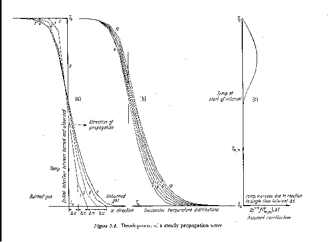
(Figure 2.), extracted
from a book published in 1955 (!) [9], shows how long such ideas have been
prevalent.
Part (b) shows how, after some time, reaction within the thickened layer causes propagation to occur, finally with uniform speed and layer thickness, into the unburned gas.
Part (c) shows the reaction-rate (plotted horizontally) versus temperature (plotted vertically on the same scale as parts (a) and (b)), which was used as the input to the calculation.
Recognised either explicitly (in MFM) or implicitly (in FLM) by the various model makers is that contact between the A and B "gas blocks" is intermittent, which is to say that, as a consequence of the turbulence, two such blocks:
Such a process is nowadays easily subjected to numerical analysis, the results of which may be represented as in the following colour plot.

What is noticeable is that the contours are symmetrical at early times, during which interdiffusion domiminates; and they become unsymmetrical later, when chemical reaction "catches up", just as was predicted by the old calculations of Figure 2.
The calculations were performed with the PHOENICS computer code, by the loading of library case 103 .
As will be explained in more detail below, it is the intermittency of these "brief encounters" which explains how volumetric reaction rate comes to be so closely connected with epsilon / k
It will also be shown that the brevity of the contact is such that, at the high Reynolds numbers that are commonly encountered, the interface layer must always be much thinner than the typical block size.
(d) The secondary reactions
Why FLM is superior to EBU is not that it is able to predict better the volumetric rate of progress of the main combustion reaction; for it is doubtful whether it can do this more often than not in circumstances of practical interest.
Its superiority lies in the fact that, through being able to estimate the distributions of the temperature and of chemical species within the interface layers, it allows calculation of the effects of secondary reactions such as those giving rise to oxides of nitrogen.
As will be shown, MFM offers the same possibilities; and in more general circumstances; and, if care is taken to ensure that comparable chemical-kinetic and transport-property presumptions are made, there is no reason why MFM should not produced the same results as FLM, for conditions for which the latter is valid at all.
(a) MFM fundamentals
The multi-fluid model of turbulence has been described in numerous recent publications [10 to 20]; and most of these, and other explanatory material, can be viewed on CHAM's web-site: www.cham.co.uk. MFM is also available for activation in the PHOENICS computer code.
Here, therefore, only the main relevant ideas will be reviewed, as follows:
(b) connections with conventional turbulence-modelling concepts
The well-known epsilon and k quantities have already been referred to. It will be useful also to connect MFM concepts with three others, namely:
These quantities are inter-related by equally well-known relationships, namely:-
Since sigma has the dimensions of 1/length, being a measure of the average thickness of the gas fragments engaging in the coupling-and- splitting process, it can be expected to be proportional to the reciprocal of Lmix,
Therefore, to avoid having to introduce another constant, let it be taken as equal to this reciprocal, so that
It is necessary to distinguish between the sigma employed in the FLM from that which is employed in MFM; for FLM pays attention only to interfaces between fully-burned and fully-unburned gases; whereas MFM recognises that the coupling-and-splitting process is a consequence of the turbulence, which disregards the chemical compositions of the materials which are brought into contact.
Thus FLM's sigma has to be zero when there is no more unburned combustible; whereas MFM's sigma can reasonably be taken as inversely proportional to Lmix, regardless of the extent of the reaction.
It is now interesting to ask two questions, namely:
First, however, it is necessary to justify the linkage of the rate of offspring production to epsilon / k by a more detailed discussion of the energy-dissipation process than has been provided anywhere in the MFM literature until now.
(c) The mechanism of energy dissipation
If, as MFM supposes, the dominant behaviour pattern of the multi-fluid population is "coupling and splitting", it must be possible to use this description to explain how turbulent kinetic energy is dissipated. Such a use of the concept now follows.
Obviously, this velocity difference is related to the turbulent kinetic energy by:
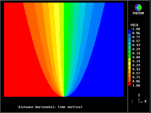
It is interesting to observe that such comparisons of MFM predictions with experiment as have been made so far have favoured a value of between 5.0 and 10.0 for CONMIX
The value most favoured by users of the Eddy-Break-Up model, is much lower, namely around 0.5; but this is easily explained by the fact that EBU is a mere "two-fluid" model, i.e. one with a very coarse "population grid".
(d) The average contact time
Since the interfacial layer grows as a result of molecular action, it is certain that its maximum thickness Llay (i.e. that which exists at the end of the "brief encounter" when "coupling" gives way to splitting) is of the order of (nulam * Tcont) ** 0.5 .
Also, the same analysis would show that the rate of production of interface material per unit volume is equal to:
It follows that:
Let now this contact time be compared with the "micro-mixing time", Tmix, defined by:
It follows that, since Re is usually much greater than unity in a turbulent flame, the contact time is much smaller than the mixing time.
One implication is that the interfacial layer does not have enough time to grow so as to have a dimension comparable with those of the "blocks" of fluid which are enjoying their brief encounter. Indeed, it can be algebraically deduced from the above equations that:
It has been remarked above, in connection with


Obviously the relevance of the epsilon/k quantity to the creation of interface material is greater if the encounter is broken off before the reactedness profile has become very unsymmetrical, i.e. before the laminar-flame propagation process has had time to dominate; so it is interesting to estimate whether this condition is likely to be satisfied.
The following argument allows this question to answered:-
The following summarising remarks about the connections between FLM and MFM therefore appear to be appropriate:
MFM also has a presumption about the profiles in the layer, as part of its coupling-and-splitting hypotheses. The only presumption which has been seriously explored so far, namely the "promiscuous Mendelian" one, implies symmetry within the inter-diffusion layer; but this can easily be remedied.
FLM requires, for validity:
These requirements are satisfied by PHOENICS Input-Library Case, L103, of which the descriptive part runs as follows.
  Stirred reactor with a 1D population distribution, and
  reactedness, ranging from zero to 1, as the population-
  distinguishing attribute.
                                                    ___________
  It is supposed that two streams of fluid         |           |
  enter a reactor which is sufficiently       A ====>          |
  well-stirred for space-wise differences          |  stirred  |
  of conditions to be negligible, but not          |  ///|/// C===>
  sufficiently for micro-mixing to be              |  reactor  |
  complete.                                   B ====>          |
                                                   |___________|
  The two streams have the same elemental
  composition; but one may be more reacted than the other.

  The flow is steady, and the total mass flow rate per unit volume
  is 1 kg/s m**3 .
The flow is zero-dimensional in the geometrical sense; but, to give it significance for a three-dimensional combustor simulation, it might be regarded as representing a single computational cell in the 3D grid. Then the conditions in the inlet streams might represent those in the neighbouring cells, from which material enters by way of diffusion and convection.
The calculations to be reported have been conducted with a 25-fluid model, and with reactedness as the population-defining attribute.
The reaction-rate-versus-reactedness formula is of the well-known kind:
where R stands for reactedness.
The exponent, CONREA2, has been given the value 5.0, which represents sufficiently well for the present illustrative purposes the temperature dependence of combustion reactions.
Stream A has been chosen as being completely unburned (R=0.0) and stream B as fully reacted(R=1.0).
Various values have been chosen for the micro-mixing constant
CONMIX and
the "pre-exponential factor" of the reactivity, CONREA2
2.2 The PDFs predicted by MFM
In the following table, the second, third and fourth columns disclose the input parameters.
The first column displays:
The PDFs appear as histograms, with:
The references to "spikes" should be noted. Comparison of the values ascribed to the height of these spikes with the also-printed "maximum ordinates" shows that they are often much larger. This is the justification for the "two-fluids-mainly" idea which underlies FLM.
The average-reactedness and RMS-deviations appear in the fifth and sixth columns.
| Figure | CONMIX | CONREA | RB | ave. R | rms. R |
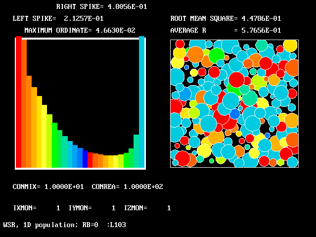 6 6 |
10.0 | 100.0 | 0.0 | 0.577 | 0.448 |
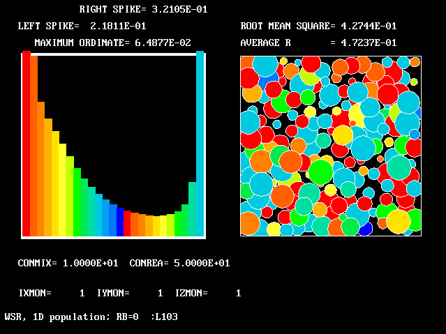 7 7 |
10.0 | 50.0 | 0.0 | 0.472 | 0.427 |
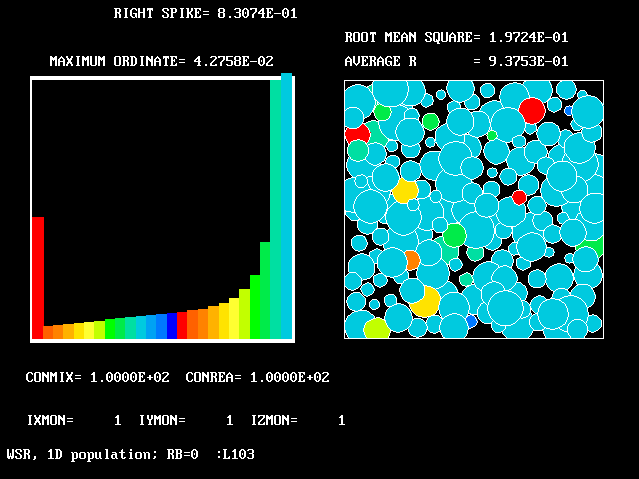 8 8 |
100.0 | 100.0 | 0.0 | 0.937 | 0.197 |
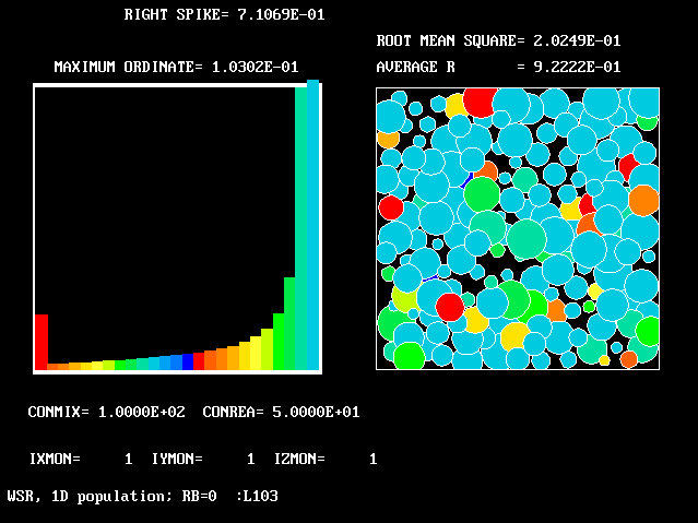 9 9 |
100.0 | 50.0 | 0.0 | 0.922 | 0.202 |
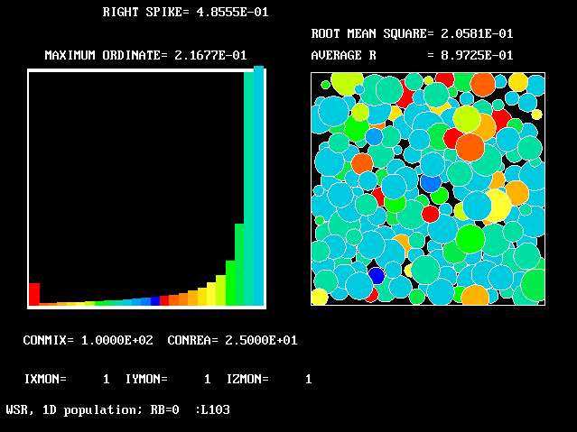 10 10 |
100.0 | 25.0 | 0.0 | 0.897 | 0.206 |
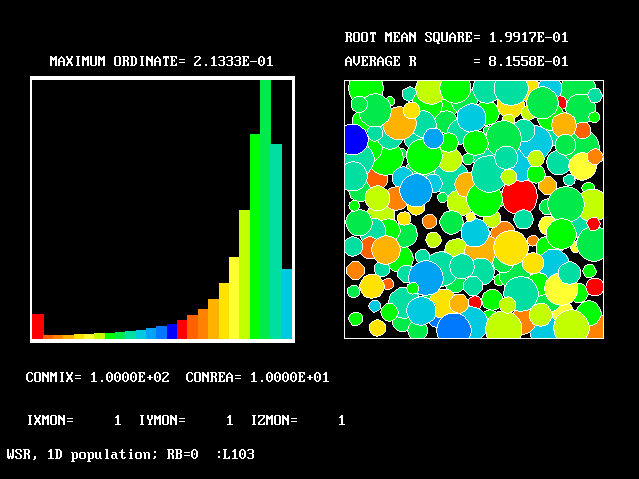 11 11 |
100.0 | 10.0 | 0.0 | 0.815 | 0.199 |
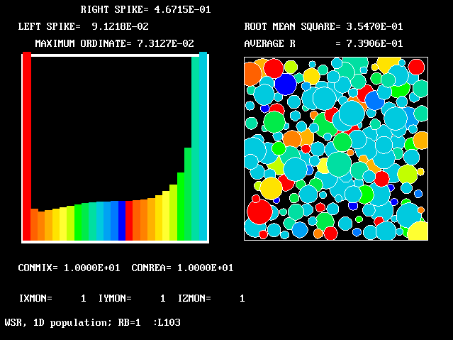 12 12 |
10.0 | 10.0 | 1.0 | 0.739 | 0.354 |
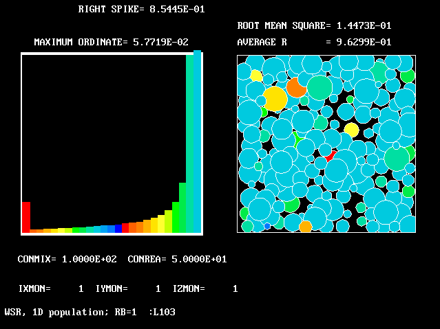 13 13 |
100.0 | 50.0 | 1.0 | 0.963 | 0.145 |
 14 14 |
100.0 | 10.0 | 1.0 | 0.927 | 0.151 |
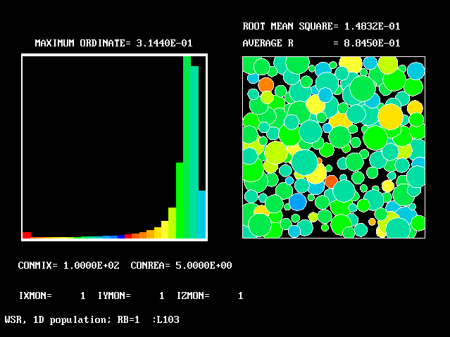 15 15 |
100.0 | 5.0 | 1.0 | 0.884 | 0.148 |
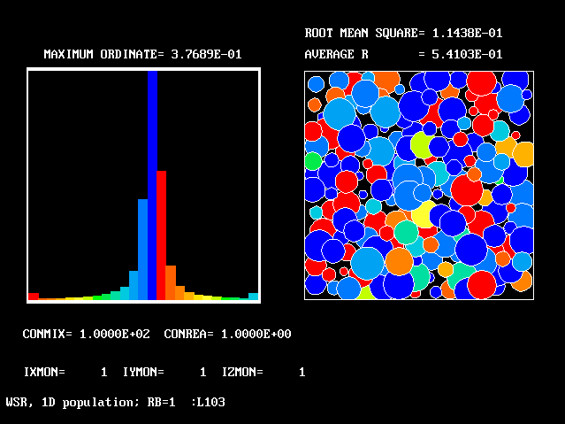 16 16 |
100.0 | 1.0 | 1.0 | 0.541 | 0.114 |
Some trends revealed by these figures will now be discussed, as follows:
In all four cases however, at least one of the spikes is large.
Any further reduction of CONREA leads, it should be mentioned, to extinction of the chemical reaction.
Understandably, the average reactednesses, for the same CONMIX and CONREA, are greater than for the RB=0 flames.
It is now possible to consider to what extent MFM confirms or contradicts the presumptions of the flamelet model of turbulent combustion.
The best confirmation of FLM presumptions is afforded by the following figures;


Whether the distributions of concentration of the intermediate gases is the same, for MFM and LFM, is another matter. As has already been indicated, LFM practitioners are inclined to believe (albeit without any closely-reasoned argument) that the distributions correspond to those of a steadily-propagating flame; whereas the foregoing analysis suggests that the transient-interdiffusion model is more appropriate.
When the following sequence of Figures is considered, support for the FLM concept becomes weaker, the last of these figure revealing a PDF which is quite unlike that which LFM presumes.


Even less supportive are the next Figures


It must indeed be concluded that FLM can be expected to represent turbulent combustion in pre-mixed gases only when the chemical reaction rate (measured here by CONREA) is large compared with the micro-mixing rate (measured by CONMIX).
This condition is perhaps satisfied for a gasoline engine, where the fuel/air ratio may be close to stoichiometric throughout; but it is unlikely to prevail for combustors into which the fuel and air enter separately.
Separate introduction of fuel and air is the subject of the next section.
(a) The cases considered
A further series of calculations has been performed for the conditions in which the two streams of fluids entering the stirred reactor have differing fuel-air ratios. Such conditions lie beyond the capabilities of the flamelet model at the present time.
Specifically, stream A has been taken as pure air; and stream B has been taken as having a fuel/air ratio of twice the stoichiometric value and a reactedness of 50 %. The two streams are equal in flow rate.
A 100-fluid model has been employed for this study, with a two-dimensional "population grid", of which the PDAs (ie population-defining attributes) are:
Further information about the definition of the model will be provided during the discussion of the results and of their displays.
| Figure | CONMIX | CONREA | average F | average R |
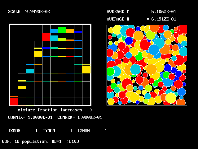 |
10.0 | 10.0 | 0.510 | 0.649 |
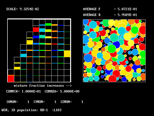 |
10.0 | 5.0 | 0.507 | 0.595 |
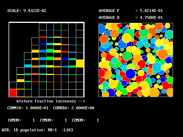 |
10.0 | 2.0 | 0.502 | 0.476 |
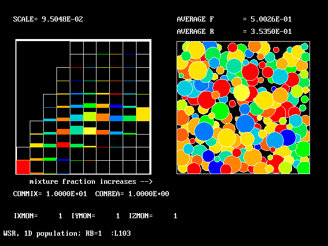 |
10.0 | 1.0 | 0.500 | 0.354 |
 |
10.0 | 0.0 | 0.500 | 0.222 |
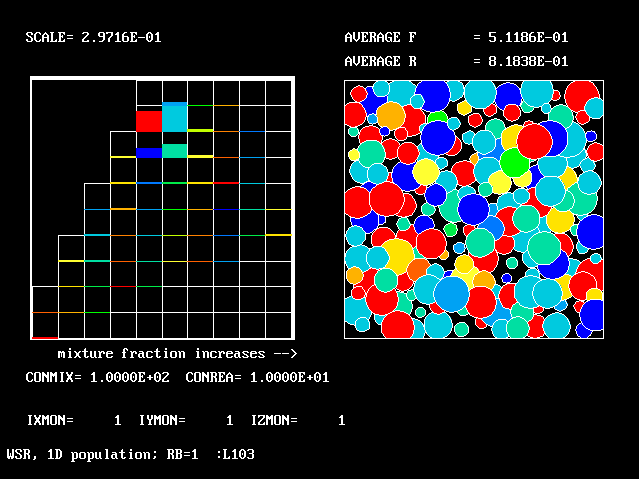 |
100.0 | 10.0 | 0.512 | 0.818 |
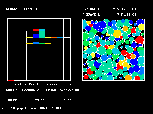 |
100.0 | 5.0 | 0.507 | 0.754 |
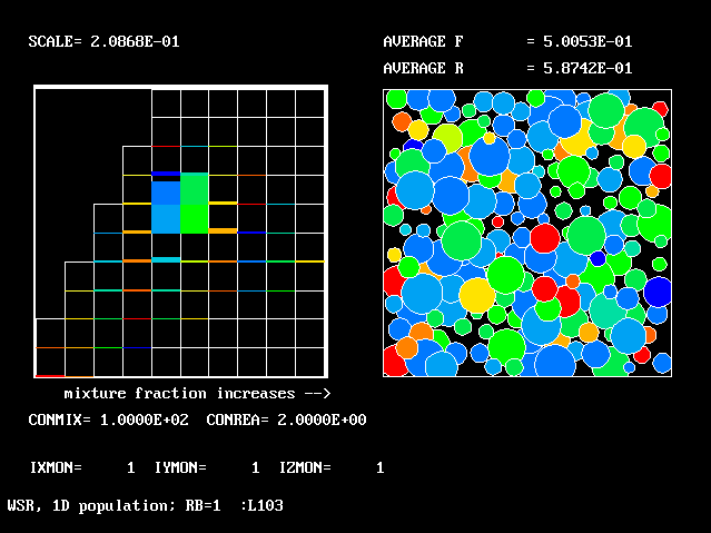 |
100.0 | 2.0 | 0.500 | 0.587 |
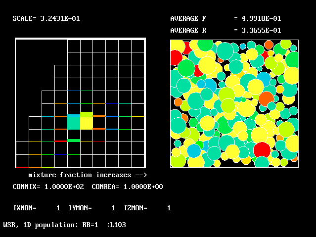 |
100.0 | 1.0 | 0.500 | 0.346 |
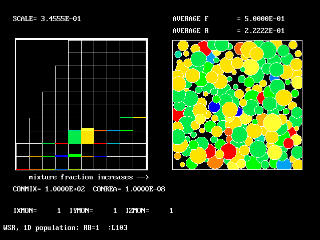 |
100.0 | 0.0 | 0.500 | 0.222 |
(b) Conclusions from inspection of the table
The runs conducted fall into two groups. The first five have the fixed CONMIX value of 10.0, and successively smaller CONREA values; and the next five have CONMIX = 100.0, and the same sequence of CONREA values.
It can be seen that:-
(c) Conclusions from inspection of the figures
All the figures have the same general form. They show a two-dimensional histogram on the left, and a graphical representation of the multi-fluid-model concept on the right.
The latter is similar to that of earlier one-dimensional population distributions; but the average-R value is printed, not the RMS deviation of F.
The left-hand diagram is however quite different from before; for it has to represent the proportions in which the total amount of material is distributed between ten fmx and ten fbu intervals.
"Spikes" no longer make any appearance.
The most-prevalent fluids are those whose "boxes" are most full of colour; the least-prevalent are those whose boxes are black.
The figures will now be discussed individually, in some detail.

When the sequence of Figure 18 to 21 is considered, it is seen that the upper (higher-reactedness) boxes are less-and-less well filled, until, when CONREA has been reduced to zero, for

Indeed, were the "population grid" finer, the histogram would provide colour only along that line.
It will have been noticed that, in all the histograms, boxes lying
to the left of the stream-A-to-stoichiometric-mixture line are
absent.
The reason is that the states represented by such boxes are not
physically attainable; for they correspond reactednesses which
exceed unity.
Therefore, although it has been stated above that a 100-fluid model is in use, the statement is a slight exaggeration; for the concentrations of fluid in the "missing boxes" are necessarily zero, and so need not be computed.
(d) Comparison between FLM and MFM for the cases considered
The above heading is included for, completeness; but there is little to say, for the simple reason that FLM, like the eddy-break-up model (EBU) to which it is the successor, is silent about mixtures of differing fuel-air ratio.
It is however worth emphasising that the "brief-encounter" model, which some writers on FLM appear to grasp, does supply the means by which "flamelet-like" concepts can be applied to turbulent diffusion flames; and it is of course the Multi-Fluid Model which provides the unifying mathematical framework.
As was mentioned at the start of the present paper, FLM is acknowledged by its proponents as being restricted in its validity to the circumstances in which the reactivity of the combustible mixtures is sufficiently high, in comparison with the turbulent mixing process, to ensure that the sum of the volume fractions of fully-burned and fully-unburned gases is close to unity.
In respect of pre-mixed (i.e. uniform-fuel/air-ratio) gases, section 2.3 has confirmed the correctness of this acknowledgement; and it has indicated that MFM permits prediction of combustion processes for which the high-reaction-rate condition is not satisfied.
When combustion of non-pre-mixed gases is in question, of the kind treated in section 3.1, the condition is hardly ever satisfied; for the "brief encounters" result in the creation of interfacial layers in which, perhaps, in some central region, the mixture ratio is near stoichiometric so that the gases are highly reactive. This must however surely be very rare; both in space and time.
It therefore appears proper to conclude that the restriction of FLM to high-reactivity conditions is a very severe restriction indeed.
The third of the limitations to which FLM is subject is that the Reynolds number must be high. This is true of MFM also, as it has been developed so far; but it is interesting to consider which of the models has the better prospect of breaking free from the limitation.
Proponents of FLM have not, to the author's knowledge, pronounced explicitly on this matter; and it is not for him to speak for them. But the following can be said from the MFM side:-
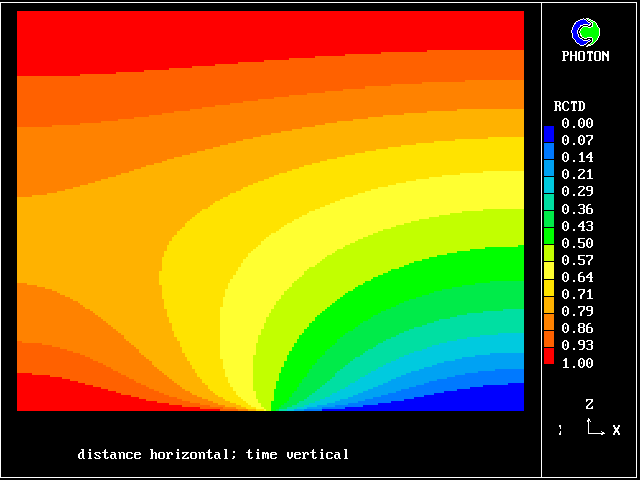
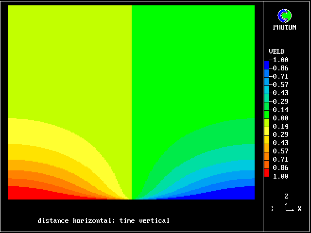
The foregoing discussion may be held to justify the following conclusions:-
by
on
organised by the Energy-Transfer and Thermofluid-Mechanics Groups of the Institution of Mechanical Engineers
at Lincoln, England, December 15-16, 1998
It is well known that, in order to predict correctly the rate of any chemical reaction which takes place in a turbulent fluid, proper account must be taken of the fluctuations of concentration and temperature.
Such account can be taken when, and only when, these fluctuations are expressed in the form of "probability-density functions" (i.e. PDFs) of the appropriate quantities; but properly-calculated PDFs are rarely used because of the computational expense of the Monte-Carlo-type methods which until recently, have been the only ones available.
Since 1995 however, the Multi-Fluid Model (MFM) of turbulence, which computes PDFs in discretised form, has greatly reduced the computational burden; and its embodiment in the PHOENICS computer code makes it accessible to design engineers.
The present paper illustrates the application of MFM to the calculation of smoke-generation rates in:
It shows that the effect of the fluctuations is very significant; and also that it can be computed with sufficient accuracy with a rather small number of fluids, and so with acceptably small computer times.
The method is recommended as being ready for experimental use by combustor designers.
Smoke is produced in gas-turbine combustors as a consequence of the thermally-induced breakdown of hydrocarbon molecules in fuel-rich regions within the flame. Since smoke production is undesirable, designers strive to reduce the extent of these regions by controlling the fuel-air-mixing process.
Computational fluid dynamics (CFD) is used for predicting the sizes and locations of such regions. However, whereas CFD can predict reasonably well the locations at which the time-average mixture ratio will be fuel-rich, that is not all that is required.
The reason is that the fluctuations of concentration and temperature which characterise turbulence entail that fuel-rich mixture is present, for part of the time, even in locations where the time-average mixture ratio is fuel-lean; and vice versa.
What is needed therefore is knowledge of the proportions of time in which, at each point in the combustor, the mixture is in the smoke-generating states; and this knowledge is obtainable only from what is called the "probability-density function" (PDF) of the mixture ratio.
Methods of calculating PDFs have been available for many years. They were conceived by Dopazo and O'Brien (1974); and Pope (1982, 1985, 1990) and co-workers have been implementing them by the use of Monte-Carlo techniques; these, however, are regarded by most combustor designers as being too expensive for regular use.
Recently, the present author has been showing, in a series of papers (Spalding, 1995, 1996, 1997, 1998), that a different mathematical method can lead to the desired information about the PDFs rather economically; and moreover that this new method has several further advantages which the Monte-Carlo technique does not.
The present paper continues the demonstrations, by considering the generation of smoke in:
The study shows that:-
There is no reason, in the author's view, for not immediately incorporating the multi-fluid model into the computer codes used by combustor designers.
2.1 The nature of MFM
The multi-fluid model (MFM) of turbulence is best regarded by those who are familiar with the Dopazo-O'Brien-Pope "PDF-transport" ideas as simply providing an alternative mathematical technique.
Specifically, it employs discretization in place of stochasticism. There is nothing especially strange about this: Monte Carlo methods can be employed for solving heat-conduction problems, even though most practitioners nowadays prefer the discretized finite-difference/element/volume methods. The same choice is available now for PDF calculations.
To those who are unfamiliar with the Monte-Carlo approach, MFM can be best regarded as applying to fluid properties, which are often thought of as "dependent variables", the same discretization techniques as are commonly applied to the "independent variables", x, y, z and time.
There is nothing new about this either. The "six-flux model" of radiation (Spalding, 1980) is of this kind; and so is the "discrete-ordinates" method (Zhang, Soufiani and Taine, 1988).
Further, particle-size distributions in multi-phase flows have long been handled by similar dependent-variable-discretization techniques (Sala and Spalding, 1973; Fueyo, 1992).
The central idea of MFM is that of a "population of fluids", the members of which are distinguished by one or more "population- distinguishing attributes" (PDAs), which are then arbitrarily discretised by the analyst.
However, each of the fluids can also possess an unlimited number of "continuously-varying attributes" (CVAs).
As far as smoke-generation modelling is concerned, the most relevant PDA appears to be the fuel/air ratio; it is therefore the one used in the present study. Other variables, such as temperature, free-fuel mass fraction, and smoke content, thus become CVAs.
It may be remarked that the distinction between PDAs and CVAs is not emphasised in the Monte-Carlo-method literature, and is perhaps not present.
The sketch
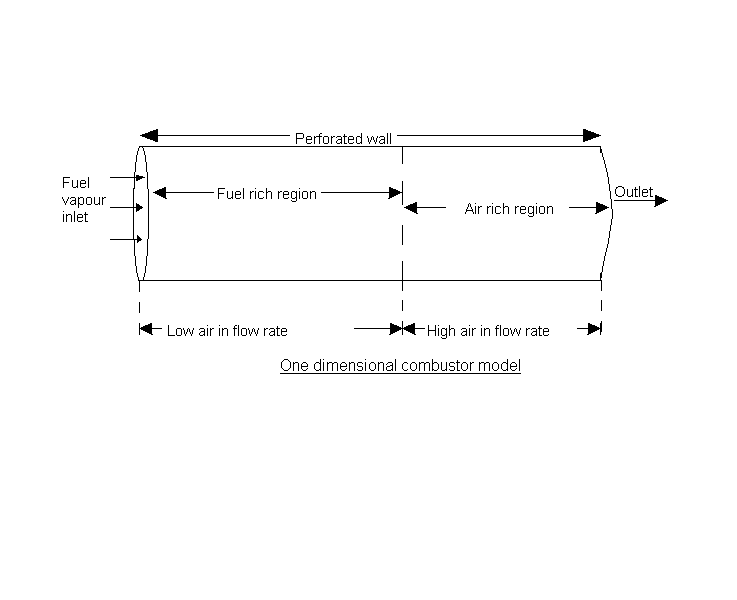
It should be understood that the one-dimensional model is employed only because it is economical and sufficient. The simulation procedure is applicable without difficulty to two and three-dimensional circumstances, and to time-dependent conditions.
Whereas the main combustion reaction is supposed to proceed in accordance with the "mixed-is-burned" rule, the smoke-generation reaction is supposed to be kinetically controlled.
Specifically, the rate is taken as being governed by the formula:
Of the two constants, the first is arbitrary, because it is comparisons which are in question, not absolute values; but the second is given values between 1 and 10, in order that the effect of the steepness of temperature dependence can be explored.
Subsequent oxidation of the smoke is not considered, because it is not relevant to the main purpose of the paper.
The calculations to be reported have been carried out with the aid of the PHOENICS (version 3.1) computer code, for which the multi-fluid model is an optional, but standard, attachment.
A grid of 50 uniform intervals was chosen for the flow direction.
Runs took between 30 seconds and 4 minutes to achieve convergence on a Pentium-200 personal computer, depending on the number of fluids employed.
No non-standard settings or additions were needed.
A typical screen dump at the end of a base-case run, shown below, reveals the smooth approach to convergence. This run lasted 30 seconds.
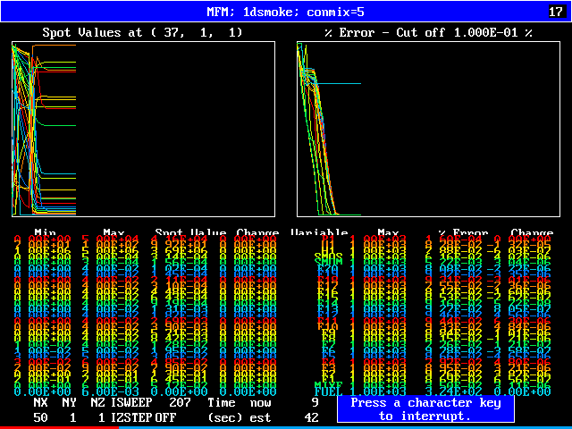
The results of the calculation will be presented, in the first instance, by way of plots with various local gas conditions as ordinates and with distance along the pipe as abscissa, as follows:
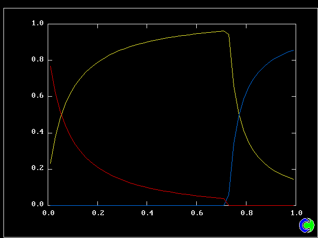
The greater steepness of the curves in the down-stream quarter of the duct is the result of the increased air-injection rate there.

Evidently the amount of smoke which will be generated, according to the multi-fluid model, is only about one half of that which the fluctuation-neglecting single-fluid model predicts.
This is because the mixture at any location consists of a population of fluids, each having its own values of:
Their distributions will be shown in the next two figures.

Understandably, the concentration of the pure-fuel fluid diminishes, that of the pure-air fluid increases, and that of the stoichiometric- mixture fluid rises and falls, with distance down the combustor.
The next sketch shows more profiles.
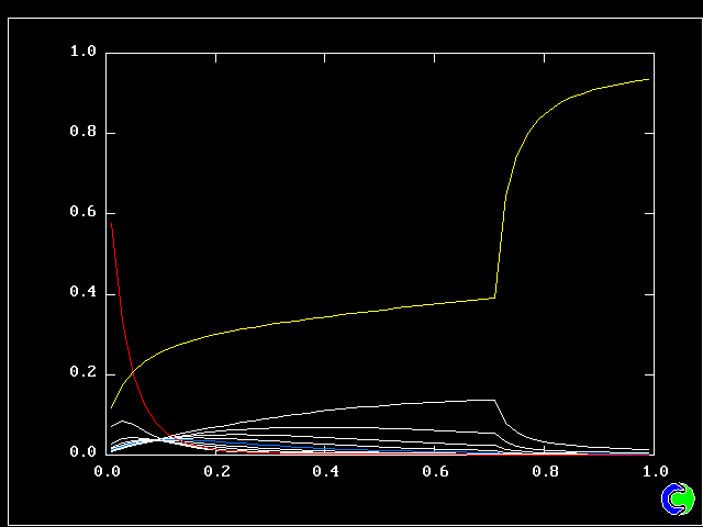
Evidently, MFM's picture of the conditions in the combustor is more sophisticated than that of the single-fluid model; and it is (qualitatively at least) certainly more realistic.
Statistical properties of the fluid population can be easily deduced; of which three now follow.
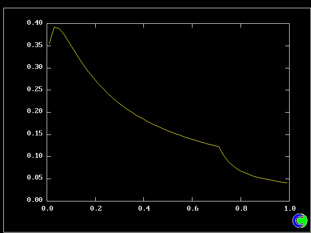
The root-mean-square fluctuations are greatest at the left-hand end, where pure fuel meets pure air. They diminish as the pure fuel disappears and fluids of intermediate fuel-air ratio come into existence.

MFM (blue curve) shows a much lower population-average temperature than the single-fluid model; for only near-stoichiometric-mixture material has the maximum temperature; and there is not much of this in the population.
This observation explains why the smoke-generation rate is so much lower for MFM.
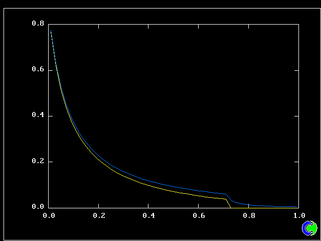
Interestingly, there is more free fuel according to MFM; and this would lead to an enlarged smoke-generation rate, were it not for the over-whelming effect of the temperature dependence.
It is also noteworthy that MFM predicts that the finite-free-fuel region extends downstream beyond the point at which the population-average mixture ratio is stoichiometric, which accords with experimental observations.
Further insight into the way in which the fluid population changes with position in the combustor is provided by the following PDF print-outs, in which the figure on the left represents the PDF, in histogram style, while the figure on the right serves simply as a reminder of the random-mixture concept which underlies MFM.
In the following list, cell 5 is near the inlet to the combustor, and cell 50 is adjacent to the outlet. indicate which computational cell is in question, out of the 50 which are provided for the whole combustor.

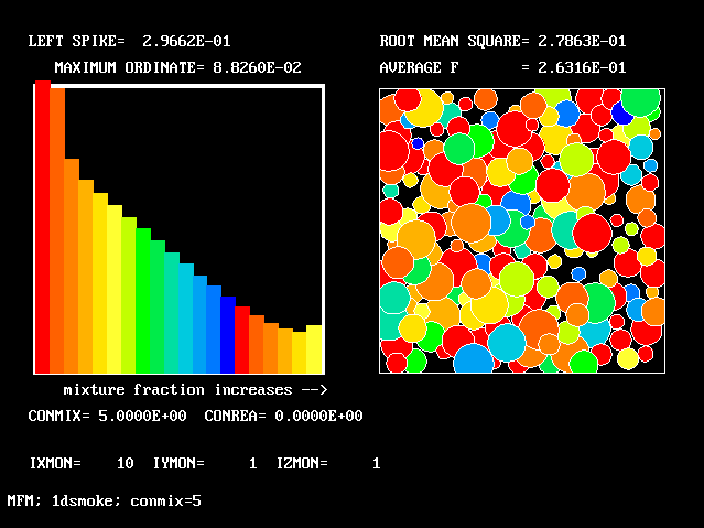


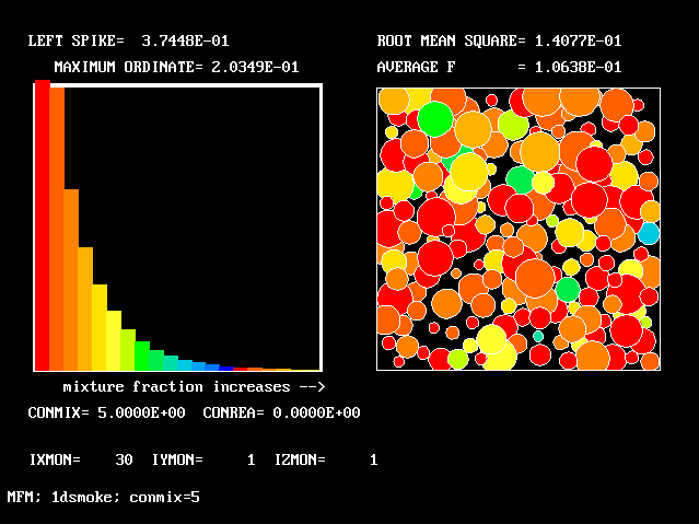
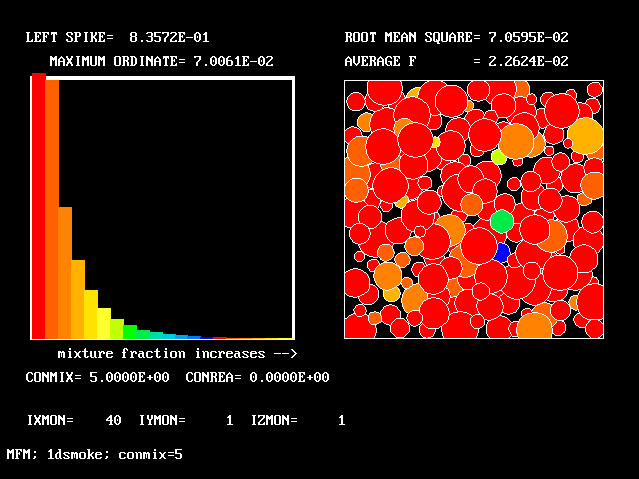
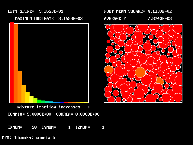
It is interesting to observe that the shapes of these PDFs are rather unlike those which are customarily presumed by those who seek to replace calculation by presumption.
Numerical data for the smoke-production rate are contained in the following table, which confirms that accounting for fluctuations predicts significantly less smoke production
SFM stands for "single-fluid model", and MFM for multi-fluid model.
| Run | CONMIX | SMOEXP | NFLUIDS | SFM rate | MFM rate |
| 1 | 5.0 | 7.0 | 20 | 6.09E4 | 3.32E4 |
Calculations have also been carried out for a range of values of the micro-mixing constant CONMIX. The numerical results are shown in the following table.
| Run | CONMIX | SMOEXP | NFLUIDS | SFM rate | MFM rate |
| 2 | 1.0 | 7.0 | 20 | 6.09E4 | 8.59E5 |
| 1 | 5.0 | 7.0 | 20 | 6.09E4 | 3.32E4 |
| 3 | 10.0 | 7.0 | 20 | 6.09E4 | 4.91E4 |
| 4 | 100.0 | 7.0 | 20 | 6.09E4 | 5.56E4 |
Increasing the micro-mixing constant, CONMIX, evidently increases smoke production. This is understandable, becaause it brings the mixture closer to the no-fluctuations state postulated by the single-fluid model.
The following pictures explain how this occurs by showing how the population-average temperature rises with CONMIX.
Population-average temperature distributions according to the single-fluid
and multi-fluid models, for CONMIX =
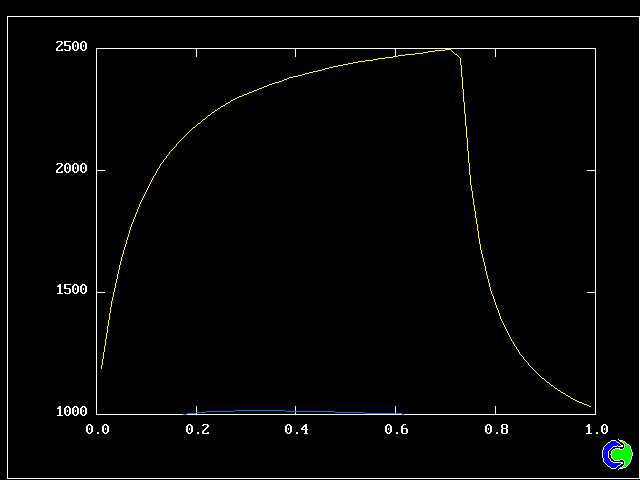

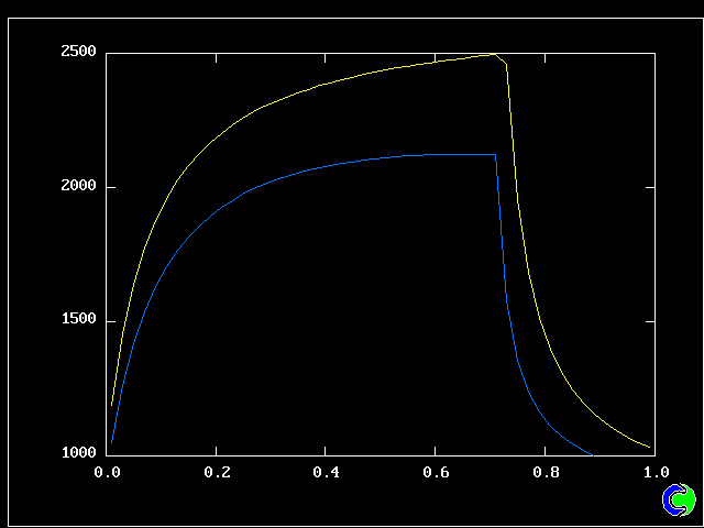
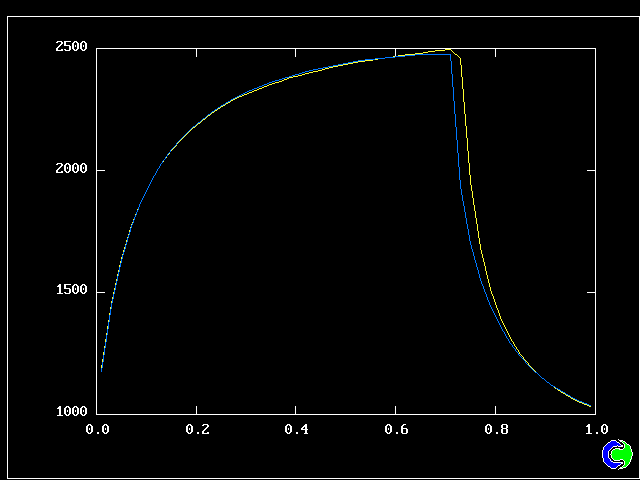
Changes in other aspects of the solution are illustrated in the following series of pictures
The smoke-concentration distributions:
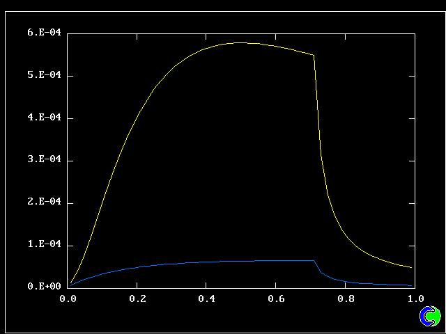

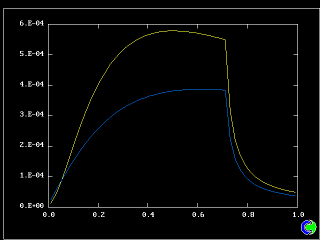
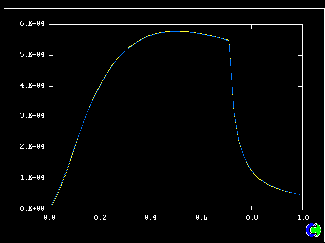
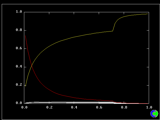

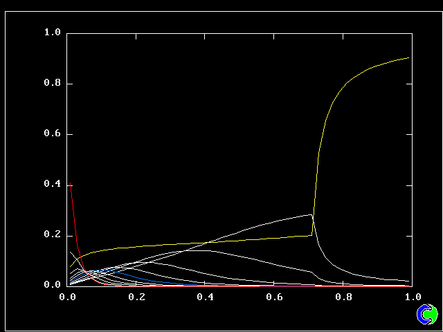
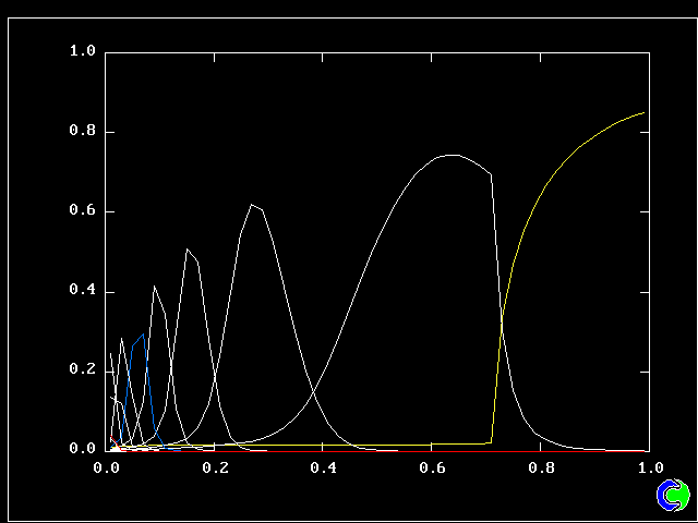
The root-mean-square fluctuations of mixture fraction:


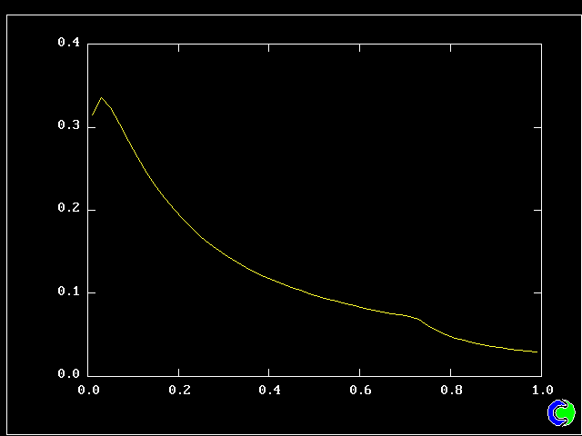
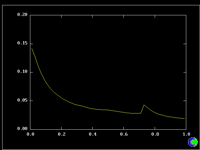
The population-average free-fuel mass fraction:


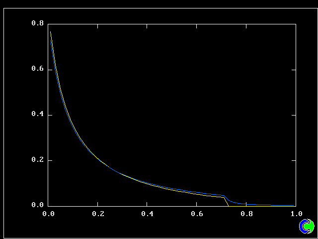

Calculations have also been made with the base-case values of CONMIX and NFLUIDS, but with greater and smaller values of the temperature-dependence constant, SMOEXP. The results are shown in the next table.
| Run | CONMIX | SMOEXP | NFLUIDS | SFM rate | MFM rate |
| 5 | 5.0 | 1.0 | 20 | 1.95E3 | 1.65E3 |
| 6 | 5.0 | 3.0 | 20 | 1.19E3 | 7.76E4 |
| 1 | 5.0 | 7.0 | 20 | 6.09E4 | 3.32E4 |
| 7 | 5.0 | 10.0 | 20 | 4.17E4 | 2.16E4 |
Evidently, increasing the temperature exponent makes the effect of fluctuations more pronounced.
The following pictures show the corresponding smoke distributions along the length of the combustor.
Mass fractions of smoke according to the single- (upper
curve) and twenty-fluid (lower-curve) models, for the temperature
exponent: SMOEXP =
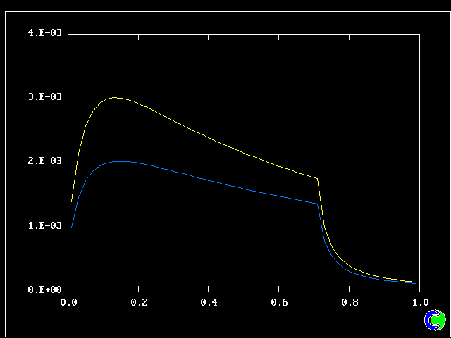
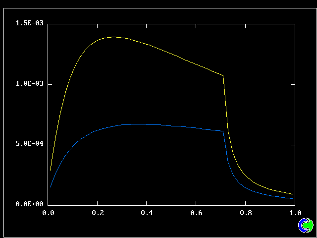


CONMIX and SMOEXP have physical significances; but, as in all CFD calculations, some purely numerical parameters may also influence the results.
In MFM calculations, the most doubtful such parameter is NFLUIDS, which measures the fineness of discretization of the fluid population.
Accordingly, some calculations have been carried out to explore its effect, with the result shown in the following table.
| Run | CONMIX | SMOEXP | NFLUIDS | SFM rate | MFM rate |
| 8 | 5.0 | 7.0 | 3 | 6.09E4 | 1.22E4 |
| 9 | 5.0 | 7.0 | 5 | 6.09E4 | 3.65E4 |
| 10 | 5.0 | 7.0 | 10 | 6.09E4 | 3.99E4 |
| 1 | 5.0 | 7.0 | 20 | 6.09E4 | 3.32E4 |
| 11 | 5.0 | 7.0 | 100 | 6.09E4 | 3.23E4 |
Inspection of this table, with the presumption that the 100-fluid value is the correct one, shows that:
Changes in other aspects of the solution are illustrated in the following series of pictures
The smoke-concentration distributions:
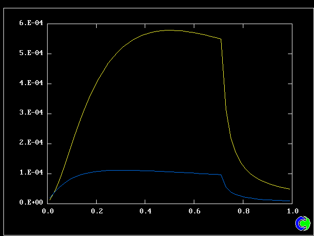
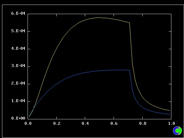


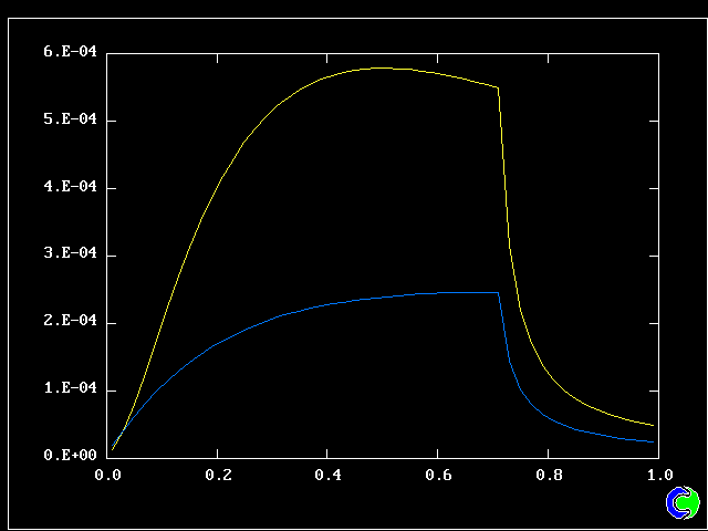
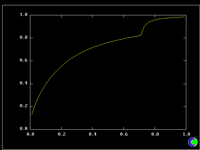
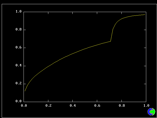


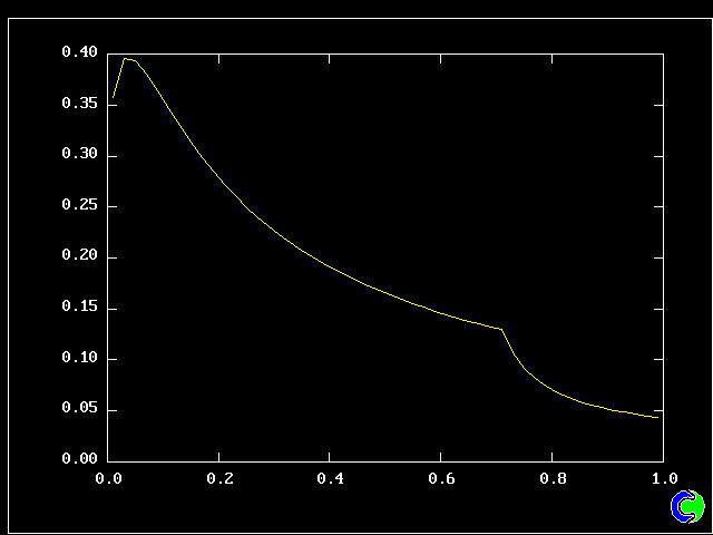
Population-average temperature distributions:
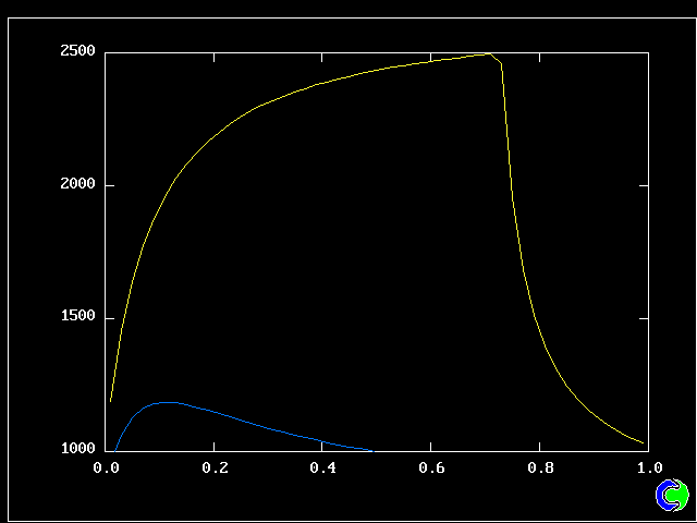
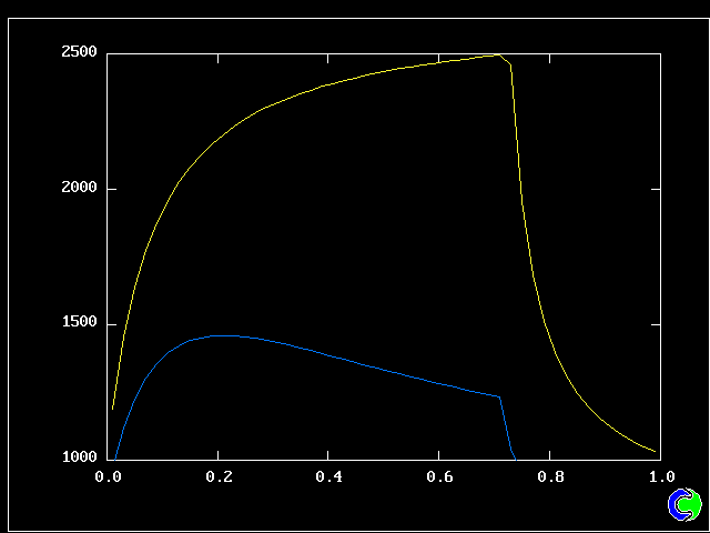
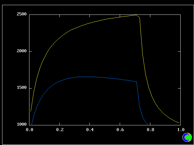

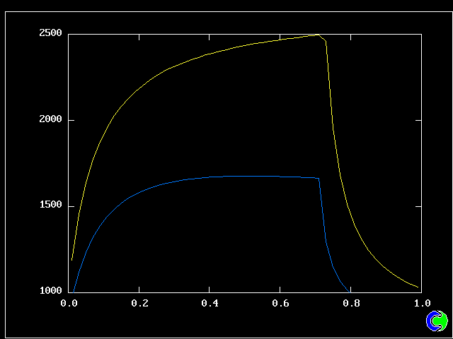
The population-average free-fuel mass fraction:
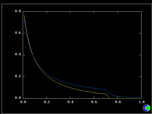
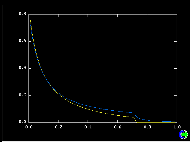


The above-reported study appears to the present author to justify the following conclusions:-
The same smoke-generation model has been activated for case 492 of the PHOENICS input-file library, which represents a (rather simple) three-dimensional gas-turbine-like combustor, which is fed by a rich-fuel-air vapour mixture, and primary-, secondary- and dilution-air streams.
The grid is coarse, namely 6*10*13 for a 30-degree sector; but it suffices for the present purposes, which are:-
The calculations performed have all had the same values of CONMIX and SMOEXP as in the one-dimensional study; but the number of fluids has been varied, from 10 to 50.
As will be seen, even the 10-fluid model gives a prediction which may be accurate enough for many purposes.
The graphical convergence monitor for the 40-fluid run
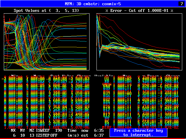
The results are tabulated in a similar manner to before; but approximate computer times are here added, as follows.
| Run | NFLUIDS | SFM rate | MFM rate | seconds |
| 12 | 10 | 7.4 E-4 | 2.38E-3 | 139 |
| 13 | 20 | ditto | 2.28E-3 | 217 |
| 14 | 30 | ditto | 2.31E-3 | 267 |
| 15 | 40 | ditto | 2.26E-3 | 485 |
| 16 | 50 | ditto | 2.27E-3 | 599 |
Two points may be remarked upon, namely:
The following figures show the computed PDFs for a location in the
middle of the outlet plane of the combustor, for:
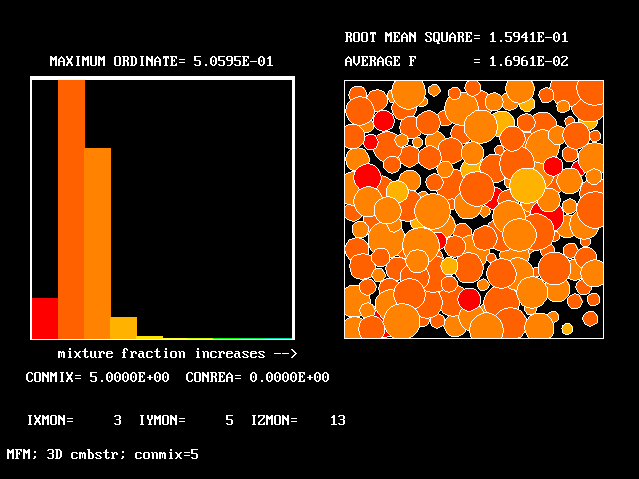
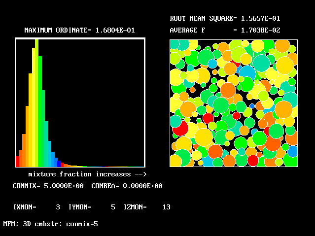

The shapes are all similar; and the root-mean-square and population-average values do not differ much.
The following contour plots show various aspects of the 50-fluid
calculation:
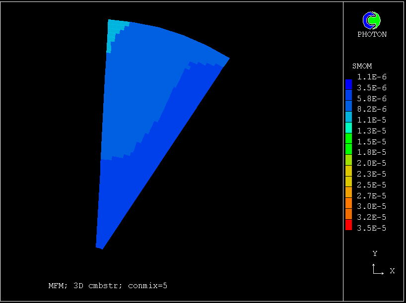
The smoke distribution on an axial plane according to:
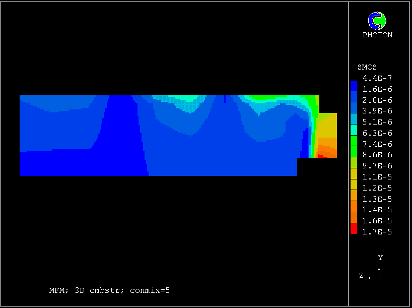
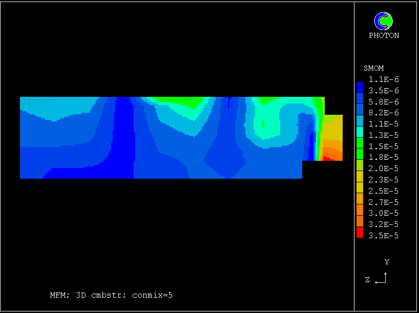
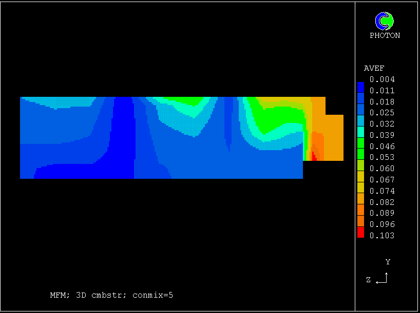

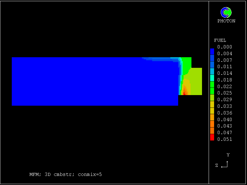
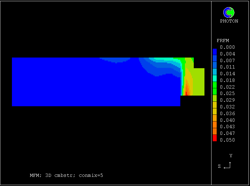
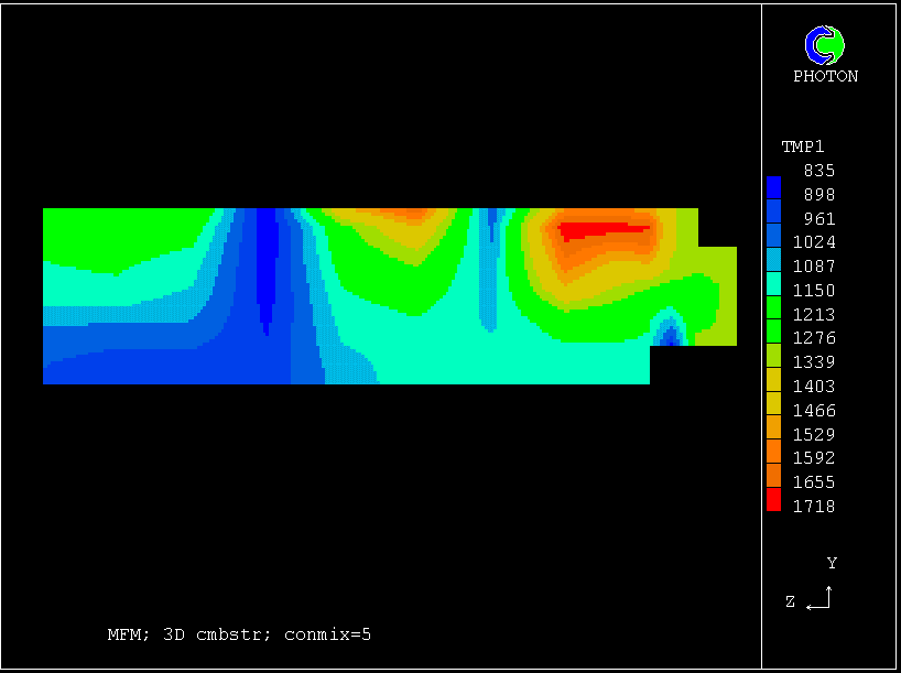
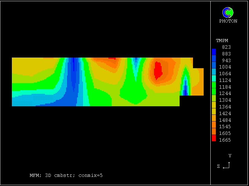
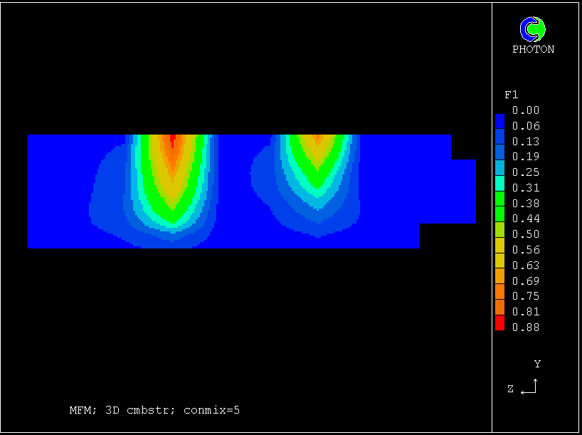


It is interesting to speculate as to why the one-dimensional study showed MFM to predict less smoke than SFM, while the three-dimensional study showed the opposite. At least two reasons may have had an influence, namely:
The second observation represents a contrast with typical engineering practice, in which very large numbers of geometrical cells are employed, in the hope of procuring high accuracy; but this hope is rendered vain by the conventional employment of far too coarse a population grid.
Thus, in practice the fluctuations are ignored, as when a single-fluid model is is used; or some version is utilised of the eddy-break-up model, which in MFM terminology, is just a two-fluid model.
What is desirable, of course, is to maintain a proper balance between the two kinds of discretization. MFM allows this.
by
Computational fluid dynamics has been used for predicting the perfomance of gas-turbine combustors since the early 1970s; but its more extensive use is hampered by two main factors, namely:-
This lecture concerns the first of these; and it explains how a newly-developed "cut-cell" technique, called PARSOL, enables curved-surface geometries to be adequately handled by easy-to-create cartesian or polar grids.
Coupled with another available technique, namely fine-grid-embedding, PARSOL may provide an acceptable solution to the grid-generation difficulty.
PARSOL has already been incorporated into PHOENICS, as has fine-grid-emedding; and some applications to combustion-chamber flows are described in the lecture.
PARSOL is however still being developed further. Some of the started and planned further features are described.
(a) The historical perspective
Computational fluid dynamics has been used for predicting the perfomance of gas-turbine combustors since the 1970s, the earliest paper known to the author being Reference 1, in which a 7*7*7 (!) grid was used to solve the equations for:
The SIMPLE algorithm was used for solving the coupled hydrodynamic equations; and the mixed-is-burned hypothesis was employed.
At around the same time, the first papers were being published on how the influences of the turbulence on the chemical reaction might be taken into account, by way of the "eddy-break-up" [Reference 2] and "presumed-PDF" [Reference 3] concepts.
(b) The current situation
Current uses of CFD by combustor developers employ essentially the same quarter-century-old ideas, but with the following differences:-
Despite the advances just alluded to, the use of CFD is far from enabling extensive experimental testing to be dispensed with. The reasons are:-
The present author has addressed the latter difficulty in a two recent papers [References 10 & 11]. The present paper is therefore directed towards the first problem, i.e. that of grid generation.
(c) The main grid-generation alternatives
Adjectives distinguishing computational grids are:-
Of these, and of their advantages and disadvantages, there is much that can be said, but little that will procure agreement among the specialists.
The present author's views are:-
Recently, two developments have made the latter preference realisable. They are:-
The next section will be devoted to describing FGEM and PARSOL in general terms; thereafter applications to gas-turbine combustors will be presented.
To present the topic of this section, it is necessary to introduce several ideas in quick succession, namely:-
Legitimate conclusions from detailed inspection of the just-mentioned material appear to be:-
In order to illustrate how PHOENICS can be used for simulating flows within combustors having curved walls without use of body-fitted coordinate grids, an idealized combustor model has been created which exhibits all the main geometrical features, namely:-
The geometry has not in fact been created by means of a standard CAD package, but rather by a stand-alone Fortran-program utility which can make simple shapes very fast. However, that is not relevant to the present demonstration of the ability of PHOENICS to handle objects defined by facets, whatever their origin.
The geometry is shown in the following screen dumps from the VR editor.
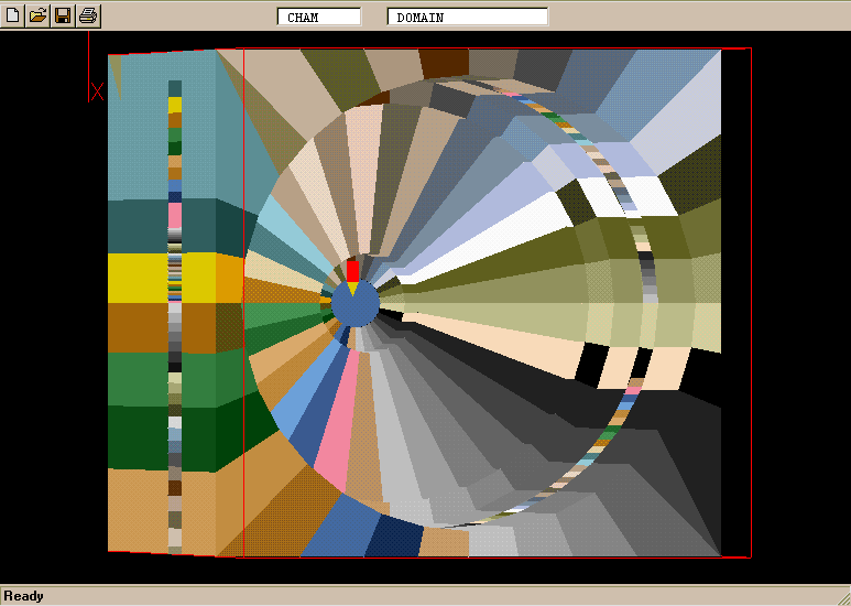
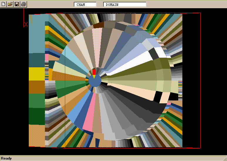
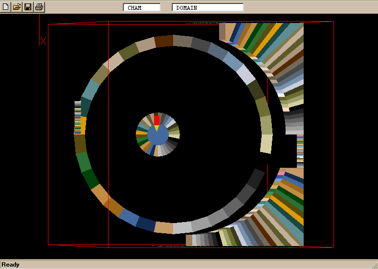
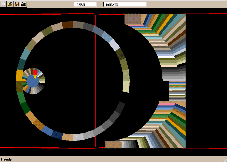
The flow is steady and turbulent, with use of the so-called LVEL model for simplicity; heat transfer results from the fact that the various streams enter at different temperature; but chemical reaction has not been activated.
The same problem has been simulated in three different ways, namely:-
(b) The grid-generation problem
On this topic it perhaps suffices to say that there is no grid-generation problem, for the user, because:
The following Figures represent various aspects of the first-stage solution, by way of "screen dumps" from the PHOENICS "Virtual-Reality" Viewer.
Noteworthy features are:
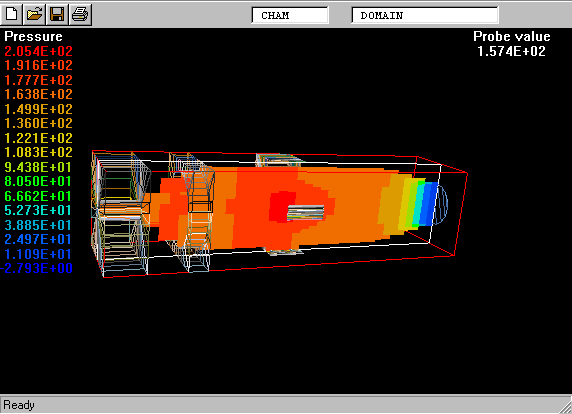
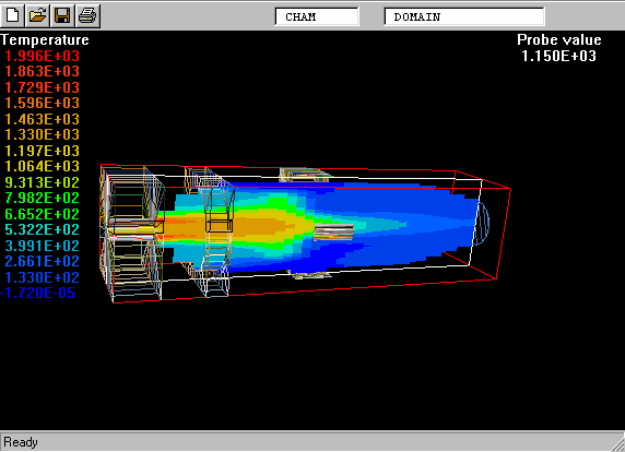
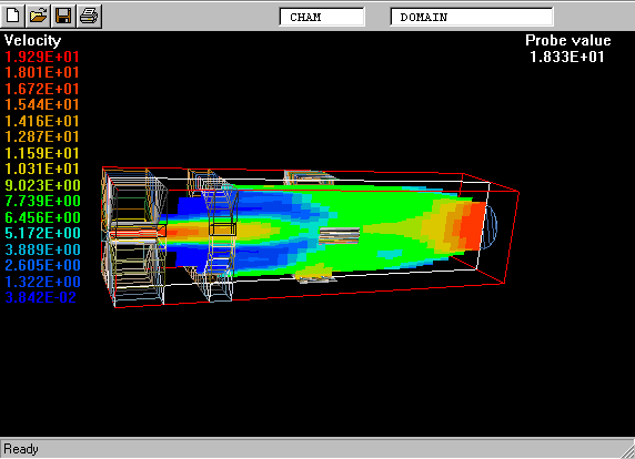
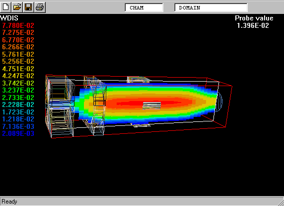
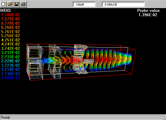
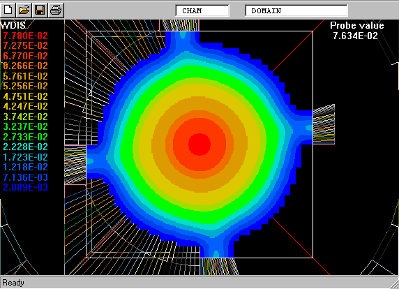
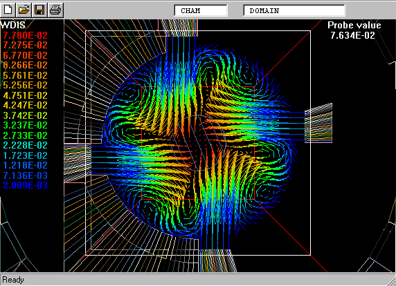
Such results, it should be mentioned, are produced by PHOENICS on a Pentium 200 MHz PC in less than half an hour.
(d) Results of the stage-2 (FGEM) calculation
The following Figures represent various aspects of the second-stage solution, by way of "screen dumps" from the PHOENICS "Virtual-Reality" Viewer.
They focus attention on the conical area enlargement, where the fine grid has been located.
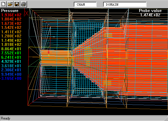
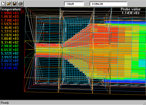
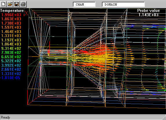
Qualitatively, the results are similar to the previous ones; but the fitting of the conical-divergence shape is obvously better because of the fine grid is embedded there.
The following further results relate to another Stage-2 calculation in which the fine-grid region is moved to the air and fuel inlet region.
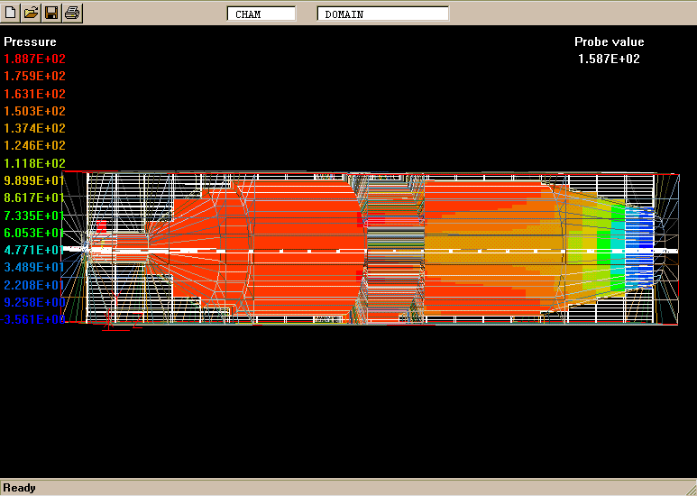
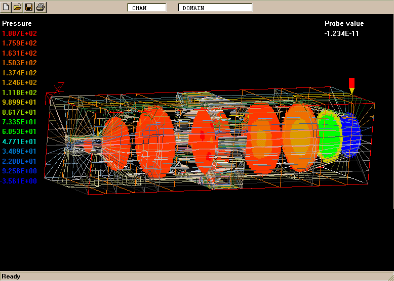
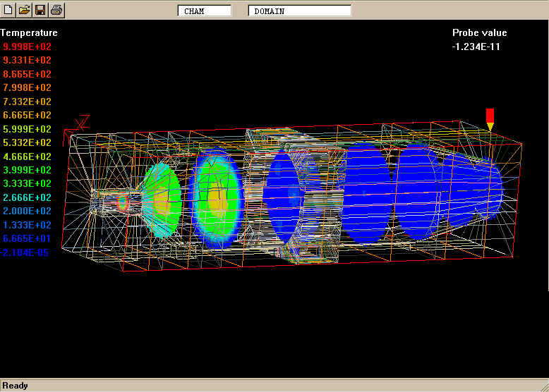
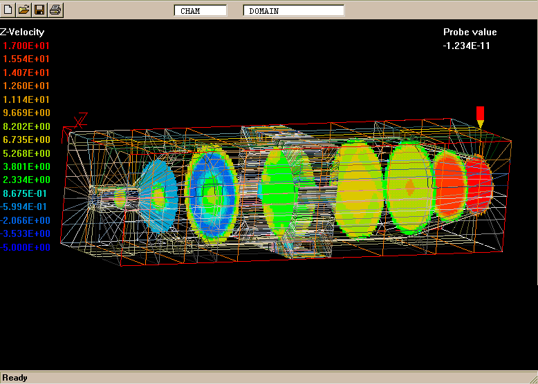
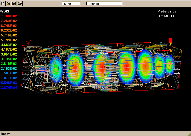
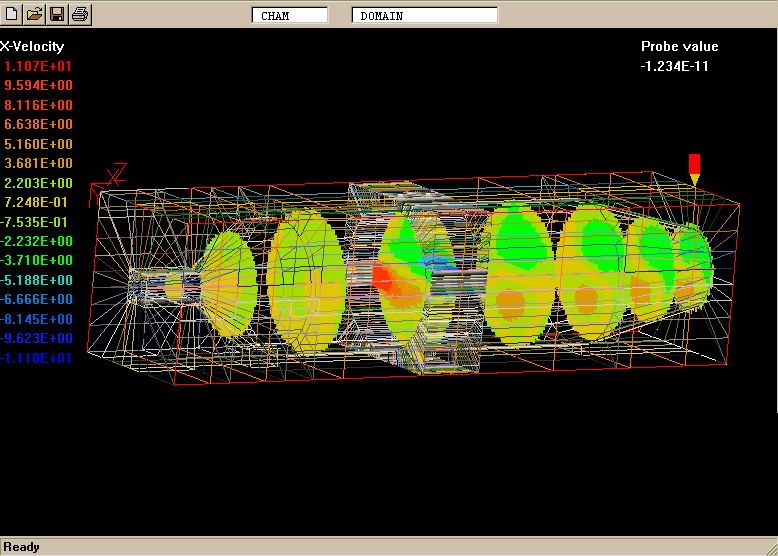
They will be left to speak for themselves.
(e) Results of the stage-3 (PARSOL) calculation
Finally a few results are shown for the case in which FGEM and PARSOL are both active.
Comparison of the contour and vector plots for the outlet cone show that the cone surface shows no significant "step effect", even though the z-direction step is still large.
Two figures which show the difference between the without-PARSOL and with-PARSOL treatments in the conical outlet region:
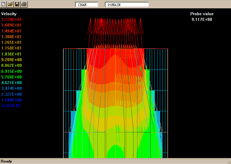
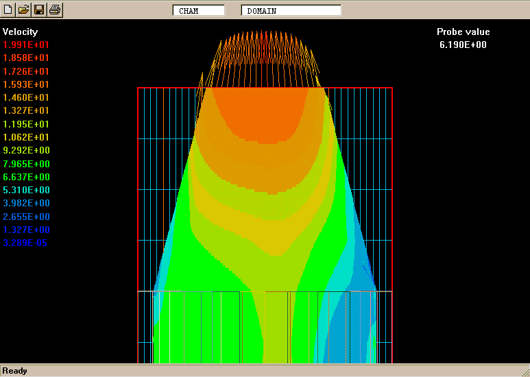
It is the latter which can be expected to be, as well as look, the more realistic.
The reasons are that:-
Fortunately, the PARSOL coding has been constructed in a modular fashion, which allows for expansion of its capabilities. Extension of its capabilities to the handling of the "thin-sloping-wall" problem is therefore now being planned by CHAM, and will be carried out during the next months.
This is not the only desirable extension. Others, for which plans are now being drawn up include:-
To the conclusions drawn at the end of section 2, it is now suggested, the following might be reasonably added:-