BFCs are particularly suitable for internal or external flows with smoothly-varying non-regular boundaries.
For such flows, BFCs provide:
BFCs can also be used to reduce numerical "false-diffusion" errors, by aligning the grid with the local flow direction where possible, e.g., for angled jets (inclined fan heater in a room)
Columns of cells must continue from one end of the grid to the other, i.e., the mesh is structured.
The cells are counted using the same conventions as in Cartesian and polar geometries:
The locations of the grid corner points must be prescribed by the user, via a Cartesian frame of axes, (XC, YC, ZC).
The alignment of the Cartesian axes - and the origin - can be chosen arbitrarily.
NOTE: The Cartesian coordinates (XC,YC,ZC) must NOT be confused with the cell-indices (IX,IY,IZ).
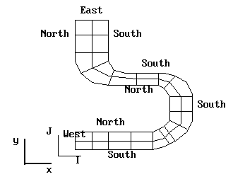
Note how the Cartesian and grid axes only coincide for the first few cells.
The compass point notation used up to now refers to the GRID coordinates, not the Cartesian coordinates.
A BFC grid is defined via the CORNER POINTS where the cell faces intersect.
The corner points are specified by their CARTESIAN COORDINATES. This may be done either
Grids generated externally to satellite can be read in by the READCO(name) command.
The corner coordinates are transmitted to EARTH via the file XYZ or XYZDA.
Note that because of the finite-volume nature of PHOENICS, there are:
So there are MORE corner points than cells.
This means that in a 2-D x-y problem (for example), you must define corner coordinates ON BOTH THE HIGH AND LOW BOUNDARY PLANES! This is often forgotten by beginners.
With BFCs, as with regular grids, scalar variables are stored at the cell center - i.e. the arithmetic mean of the cell corners.
Velocities are stored at the centers of cell faces.
The direction of the stored velocity is along the line joining adjacent cell centers.
The magnitude of the stored velocity is obtained by resolving the total velocity vector (by projection) into the direction of the line joining the cell centers.
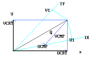
The SOLVEd velocity (U1, V1 W1) is therefore known as a RESOLUTE.
Cartesian velocity components (UCRT, VCRT, WCRT) are also calculated and stored (automatically).
These are the components of the total velocity in the directions of the reference Cartesian axes.
They should be regarded as being stored at cell centers.
Velocity Definitions
Q is the total velocity vector.
U1, V1 (and W1) are the SOLVEd velocity resolutes.
UCRT, VCRT (and WCRT) are the deduced vector components in the Cartesian coordinate system.
UCMP, VCMP (and WCMP) are the deduced vector components in the grid line directions.
Fundamentals Of Grid Generation
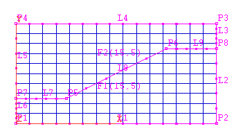
Define Nodes - The Cartesian Coordinates of all grid nodes (cell corners) must be specified.
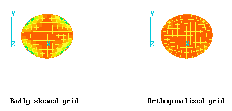
Grid Orthogonality - Lines joining cell centers should intersect the dividing face at angles as close to right-angles as possible. Angles less than about 30 degrees should be avoided if possible. This can be checked by turning the Grid check ON on the Match Grid dialog.
Grid Spacing - Grid nodes should be spaced finely where flow properties are expected to change rapidly with distance - coarsely where they don't. Smooth changes of aspect ratio are advised.
The Steps In BFC Grid Generation
The process of specifying a BFC grid involves:
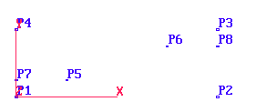
In the grid generator, POINTS are created by clicking on the 'Points', 'New Points' buttons. 'Mouse point' allows the point to be placed with the mouse, 'Type x,y,z' brings up a data entry panel.
Once created, points can be moved with the 'Modify Points' button.
The PIL command for creating points is: GSET(P,point_name,x,y,z) where x,y,z are the Cartesian coordinates of the point.
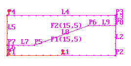
In the grid generator, LINES are defined by clicking on 'Lines', 'New Lines', then 'New Straights', New Arcs' or 'New Curves', then clicking on the points defining the line.
Once a line has been created, the number of cells along it can be set or modified with the 'Modify Lines' button.
The PIL command for a line is: GSET(L,line_name,point_1,point_2, ....)
The precise form of the command depends on the type of line.
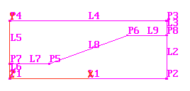
A FRAME is a four sided figure. Each side may be made up of several lines.
The number of cells on opposite sides of a frame MUST match.
In the grid generator, frames are created by clicking on 'Surfaces ', 'New Frames'. You then click on all the points making up the frame in turn. These points must already be connected with lines. When you click on the first point again, the frame is created. If the frame is made up of more than four points, you must now click on the ones you wish to be the corners.
The PIL command for creating a frame is: GSET(F,frame-name, ....
The total number of cells in each of the I, J and K directions must be specified. This is often the sum of the frame edges in each direction.
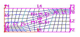
The physical dimensions of the default grid can also be set. The default grid is a rectangular block, which is then fitted, or matched, into the frames.
In the grid generator, this function is performed by the 'Dimension'button.
The PIL command for setting the grid dimension is: GSET(D, ....
Each FRAME must be matched to a portion of the mesh. You must specify the I, J, K location that the first corner is to be matched to, and indicate the direction (+/-I, +/-J, +/-K) from the first to the second, and second to third corners.
In the grid generator, this is done with the 'Surfaces', 'Match Grid' button. Click on the frame to be matched, then fill in the table accordingly.
The PIL command for matching a frame is: GSET(M,frame_name, ...
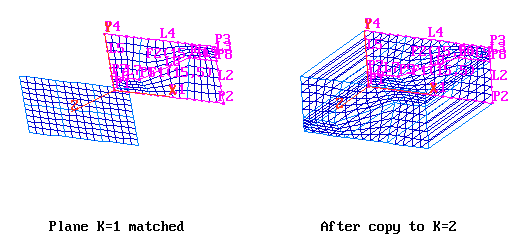
The 3-D grid can be made up from 2-D planes by:
All of these operations are performed from the 'Volumes' button of the grid generator.
The PIL commands are:
Sources Of Further Information
There is a sequence of tutorials showing all the stages of BFC grid generation.
A further tutorial on the PIL aspects of grid generation is also available through POLIS.