TR211: GENTRA User Guide Chapter 2

2. The GENTRA Input Menu

About this chapter

As noted in Chapter 1, GENTRA is equipped with three user-interfaces:
- A data-input menu;
- The use of PIL commands in the Q1 file;
- The use of FORTRAN in subroutine GENIUS.
This chapter explains how to use the input menu for problem specification. The use of the GENTRA Input Library of simulations is also discussed at the end of the chapter.
About the GENTRA Menu
1. What the GENTRA menu does
  (a) The GENTRA menu allows the user to specify the input data for the disperse phase as choices from a set of hierarchically-organised menu panels. On-line help is available to assist the user in the selection process.
  
  (b) The GENTRA menu makes, automatically, all the other provisions needed for the EARTH run. Chapter 3 of this Guide details the nature of these provisions for the benefit of the expert user.
  
  (c) The GENTRA menu writes, at the end of the current Q1 file, and as PIL commands, the results of (1) and (2) above.
2. How to access the GENTRA menu
  The GENTRA menu is accessed from the ‘Models’ page of the VR Main Menu, which in turn is accessed by clicking on the Menu button of the hand-set. Full details of the VR Environment are given in TR326: PHOENICS-VR Reference Guide.
  
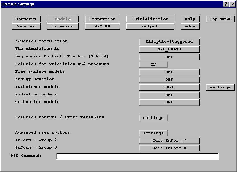
  Figure 2.1 Main Menu – Models
  
  Turn GENTRA on by clicking on ‘OFF’ next to ‘Lagrangian Particle Tracker (GENTRA)’. A new button labelled ‘Settings’ will appear. To enter the GENTRA Menu, click on ‘Settings’
3. When to call the GENTRA menu
  As pointed out in Section 2.2.1, the GENTRA menu is used to specify data for the disperse phase; the user must, additionally, specify the data for the continuous phase. This can be done in any of the ways that are available in PHOENICS, for instance:
  
  (a) By using another menu system, such as the Main Menu;
  
  (b) By entering the PIL commands directly in the Q1 file; or
  
  (c) By loading a case from the PHOENICS Input Library.
  
  The provisions made by the GENTRA menu will depend on the continuous-phase set-up (for instance, the auxiliary storage allocated by the GENTRA menu for the GENTRA-EARTH run will depend on the dimensionality of the problem). For this reason, you are advised to enter the GENTRA menu after the continuous-phase settings have been effected.
4. Obtaining help
  All the menu options have associated help entries. To obtain help on an option, click the question mark "?" at the top right corner of the dialog box, then click on the item in question.
The GENTRA Main Menu panel

If you are following the worked example provided in this chapter, enter the PHOENICS-VR environment. Click on the PHOENICS icon on the desktop, or click on Start, Programs, PHOENICS, PHOENICS. Load the PHOENICS Library Case B534 by clicking on ‘File, Load from Libraries’, entering B534 and clicking 'OK'. This case simulates the flow of a liquid (water) through a ball valve, and will be used as the basis of the worked example. Particles (e.g., solids in suspension) will be included in the flow simulation by means of the GENTRA Input Menu.

After loading the case, you can inspect the settings by double-clicking on the various objects to bring up their Attribute dialog boxes, and check the domain settings by clicking on ‘Menu’ on the hand-set.

Once you are ready to move on to GENTRA, click on ‘Menu’ on the hand-set, then on ‘Models’, turn GENTRA ON and click on ‘Settings’.

After loading the GENTRA menu as detailed in Section 2.2, the first menu panel to appear on the screen is the GENTRA Main Menu Panel, shown in figure 2.2. The options in this panel can be divided into two groups:

The first group includes options for the entry of data of four kinds:
- Particle physics,
- boundary conditions for particles,
- numerical controls and
- input/output controls.
The second group (with just one option) gives access to general information on GENTRA and the menu.

The options in these groups will now be explained in this manual. Section 2.4 below will explain what help and information are available on-line. Sections 2.5 to 2.9 will deal with the first group (i.e., data entry); and Section 2.10 will explain how to finish the menu session.

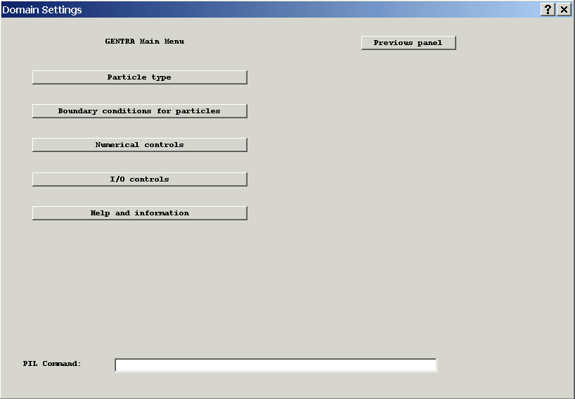
Figure 2.2: The main menu panel

Help and information

The option Help and information of the Main Menu (figure 2.2), brings up the menu panel shown in figure 2.3.

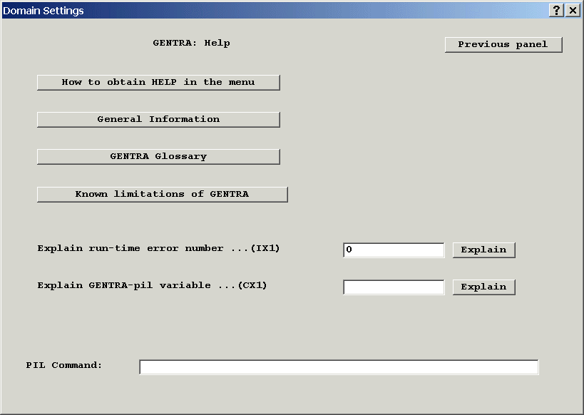
Figure 2.3: Help and information

The options in this panel are explained below.

How to obtain help in the menu. Help in the GENTRA menu is available at two levels:

1 Help on each menu option can be obtained as explained in Section 2.2.4 above.

2 Help items on special topics are available as choices from the menu. For instance, all the options in the current menu panel are informative ones.

General information. Choose this option to obtain basic information on the use of the GENTRA Input Menu. (The information contained in this menu entry is covered by several sections in this Guide.)
GENTRA Glossary. This entry contains an explanation of the terms used in GENTRA and its documentation.

The GENTRA Glossary has been included in this Guide as Appendix H.

Known limitations of GENTRA. This entry contains a list of the limitations of GENTRA which are known to the GENTRA Development Team. The list is not intended to be exhaustive; but the main limitations are presented and, where possible, alternatives are suggested.

The information contained in this entry is listed in this Guide as Appendix E

Explain run-time error number. GENTRA-EARTH will trap, at run time, a large number of error conditions, and will issue a message to inform the user. The message contains an error number and a short explanation of the error. After entering an error number and clicking Explain; a fuller explanation of the error and (if appropriate) avoidance instructions will be provided for that error.

GENTRA errors are classified into:-

Warnings (with numbers between 001 and 299), which do not abort the program but reset some of the user-supplied parameters, that are detected to be inconsistent;

Fatal errors (with numbers between 300 and 599), which abort the program;

Internal errors (with numbers between 600 and 899), which should be referred to CHAM.

By default, all the error messages are written to the screen, but you can change this in the GENIUS subroutine. Section 5.3 below provides details.

Explain PIL Variable. As an alternative to the menu, users can also specify the GENTRA settings using a subset of PIL variables (see Chapter 3 for details). Enter a variable name then click Explain. Concise reference information will be displayed.

The information provided is summarised in Appendix B of this Guide.

Previous panel. This option returns the user to the previous menu panel. This button is common to all the GENTRA menu panels.

* If you are following the worked example, you can now explore all these sources of information if you so wish, and return to the GENTRA main menu.

Particle type

The option Particle type of the Main Menu (figure 2.2), allows you to specify the type of particle (e.g., vaporising droplet, melting particle, etc); and the physics of the particle type (e.g., drag law, specific heat, buoyancy effects, turbulent dispersion).

When you choose this option, the menu panel in figure 2.4 is produced. The options in the panel are now dealt with in successive subsections.

* Click on Particle type now.

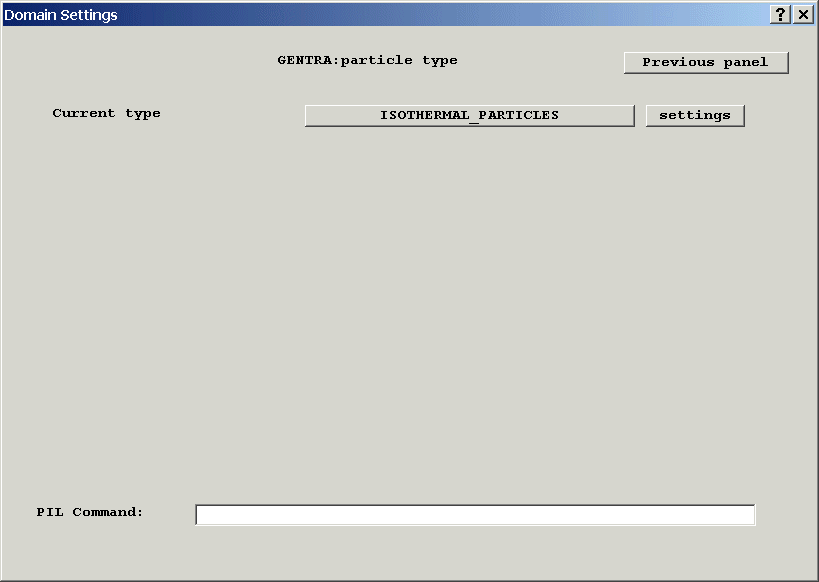
Figure 2.4: Particle type

The particle type to be simulated is selected by clicking on the name of the particle type, which by default is Isothermal Particles. This displays a list of available particle types, shown in Figure 2.5. The settings button allows the specification of the physics and data of the chosen particle type. Finally, there is an option to return to the previous menu.

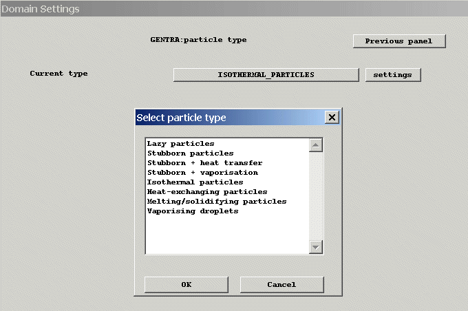
Figure 2.5: Particle type selection

* For the worked example, the isothermal particle type should be selected. The number of inputs for this particle type is small, but permits the typical features of all panels to be examined.

Lazy particles (Vpart = Vfluid). "Lazy" particles do not have a velocity of their own, but share, at each point, the continuous-phase velocity. They therefore behave like tracers.

Lazy particles do not have a size or a temperature, and cannot undergo any physical process (such as solidification, or vaporisation) though turbulent dispersion is permitted. Lazy particles have no effect on the continuous-phase solution.

On hitting a wall or obstacle, the lazy particle will be removed from the domain.

Stubborn particles (Vpart = const). "Stubborn" particles have a constant velocity, independent of the continuous-phase conditions. They therefore behave like "beams" or "rays".

Stubborn particles do not have a size or a temperature, and cannot undergo any physical process (such as dispersion by turbulence, or solidification, or vaporisation). They do not exchange momentum with the continuous phase.

On hitting a wall or obstacle, the stubborn particle will be removed from the domain.

Stubborn + heat transfer (Vpart = const). "Stubborn + heat transfer" particles behave like "Stubborn" particles, except that they can exchange heat with the continuous phase.
Stubborn + vaporisation (Vpart = const). "Stubborn + vaporisation" particles behave like "Stubborn" particles, except that they can exchange heat and mass with the continuous phase.
Isothermal particles. Isothermal particles are modelled by Lagrangian equations for the particle position and velocity, but not for the particle temperature or size. Therefore, this type of particle should be selected when no exchange of heat or mass between the continuous and the disperse phase is to be considered.

On hitting an obstacle, an isothermal particle can either be removed from the domain or bounced with a user-supplied restitution-coefficient.

Heat-exchanging particles. Transfer of momentum and enthalpy between the continuous and disperse phases is accounted for when heat-exchanging particles are employed. The particles are modelled by Lagrangian equations for the particle position, velocity and temperature.
Melting/solidifying particles. Melting/solidifying particles are modelled in a similar way to heat-exchanging particles. However, the Lagrangian equation for the particle temperature includes the effects of solid-liquid and liquid-solid phase change, and the particle diameter is determined as a function of the proportion of the solid and liquid phases present.
Vaporising droplets. Vaporising droplets are modelled by Lagrangian equations for the particle position, velocity, temperature and mass. Exchange of momentum, enthalpy and mass between the disperse and continuous phases is included.

The choice of a particle type should normally be your first action when using the GENTRA Menu, as some of the menu options (e.g., those concerning physical data or particle-obstacle interaction) will depend on the type of particle.

Physics of current particle type

The settings button on the Particle type panel enables the user to specify values for the particle physics (such as drag law, Nusselt numbers, specific heat, buoyancy effects, turbulent dispersion).

The data items to be supplied are dependent on the particle type selected in the previous menu panel. The user is therefore advised to select the correct particle type before visiting this data section.

The following subsections describe the data panels for each of the available particle types.

Data for lazy particles

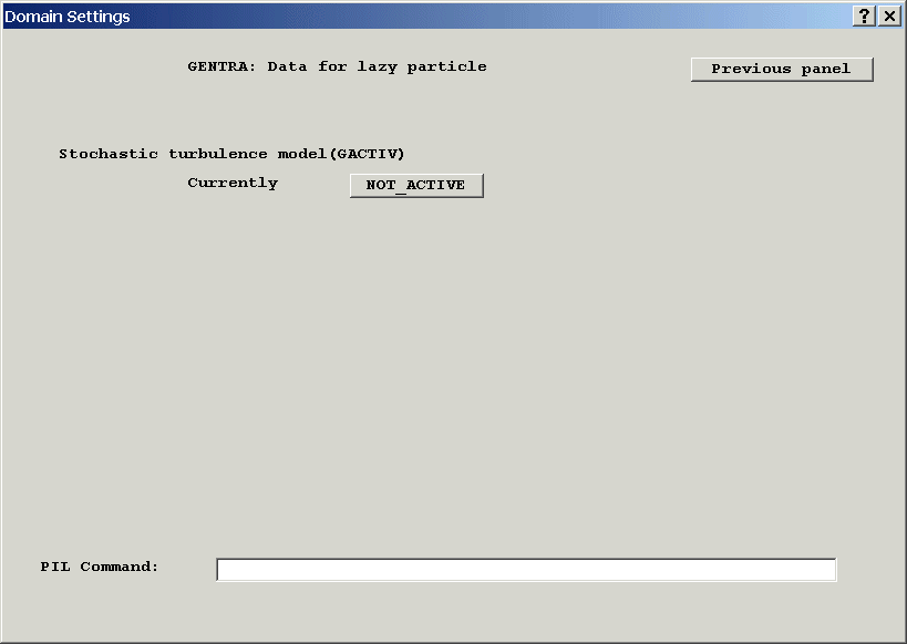
Figure 2.6: Data for lazy particles

The only data required for lazy particles concerns the use of the stochastic turbulence model for particle dispersion.

GENTRA has a built-in model that simulates the effect of the turbulent fluctuations of the continuous-phase velocity on the dispersion of particles.

The selection of the option Stochastic turbulence model in the Particle physics menu (figure 2.6) will alternately activate/deactivate this feature.

* Try this now by clicking not_active; the stochastic turbulence model will be activated. Click active, and it will be deactivated again. Then return to the GENTRA main menu panel by choosing Previous panel.

Note that, for the stochastic model to be available, the k-e model of turbulence must be used. GENTRA-EARTH will automatically deactivate it if KE and/or EP are not SOLVEd for or, at least, STOREd.

When the stochastic turbulence model is selected, the particle trajectories will be calculated from the sum of the mean continuous-phase velocity and an instantaneous turbulent velocity fluctuation determined from the local turbulence conditions.
Data for stubborn particles
No additional data is required for this particle type.

Data for isothermal particles

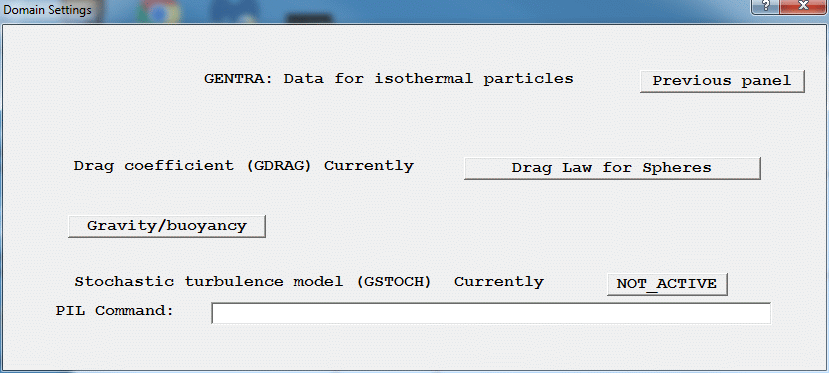
Figure 2.7: Data for isothermal particles

The drag coefficient (which is responsible for the exchange of momentum between the disperse and the continuous phase) can be specified in one of three ways:-

If a constant is used, the drag coefficient will be taken as equal to that constant.
Special flags can be used to specify laws. The built-in laws and associated flags are as follows:

Flag	Law
GRND1 (or -10120.)	Solid spheres
GRND2 (or -10130.)	Drag coefficient read from table

(See Chapter 6 of this Guide for mathematical expressions)

You can introduce your own law in Section 1 of GPROPS (see Chapter 5 for details). Recompilation and re-linking of EARTH is needed after the modification of GPROPS.

The various forms of Drag Law are selected from a menu:

Figure 2.7a: Selecting the Drag Law

When the 'Drag Law from table file' option is selected, the dialog offers buttons to:

create a new, empty, file
select a pre-existing file, or
open the selected file in a file editor for inspection and modification.

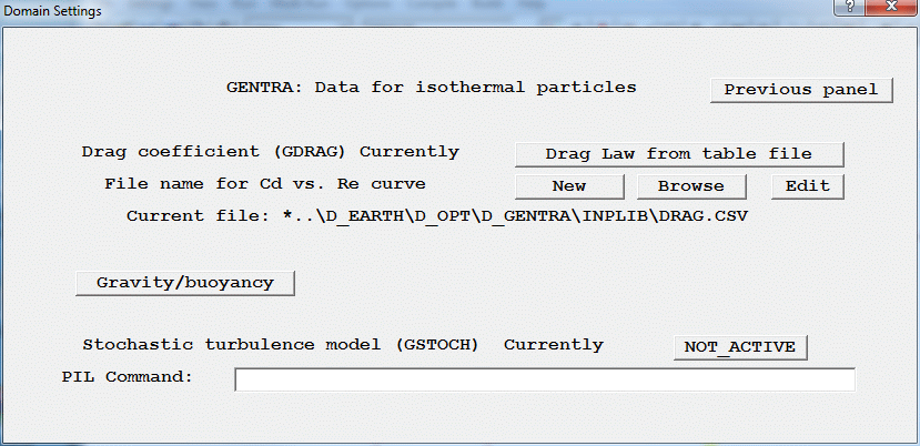
Figure 2.7b: Drag Law from table file

The file should contain two columns of numbers. The first is the Reynolds Number, the second the Drag Coefficient at that Reynolds Number. There is no limit to the number of lines. Blank lines, lines starting with # and anything after ! is ignored. The first active line can optionally contain headers for the columns. The columns can be separated by blanks, comma (,), semicolon (;) or tab. An extract from the example file, which gives the same Cd-Re relationship as the 'spheres' expression, is given below:

# Drag curve for spheres, taken from Clift, Grace & Weber
# as implemented in GENTRA 
# https://www.cham.co.uk/phoenics/d_polis/d_docs/tr211/chap6.htm#6.3
# Valid for rigid spherical particles up to Re<3E5
Re   , Cd
1.8  , 16.38612019
9.61 , 4.346219022
23.4 , 2.44605341
43.2 , 1.742424078
68.7 , 1.386829359
98.9 , 1.177059906
134.0, 1.036072042

* The built-in law will suffice for the worked example. However, you can enter other values, then enter GRND1 again for the sake of practice. Then return to the previous panel by clicking Previous panel.

The gravity/buoyancy forces option enables the user to activate gravity forces for the particles, and to include buoyancy and pressure gradient effects. The option brings up the menu panel displayed in figure 2.8.

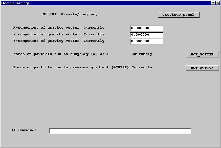
Figure 2.8: Gravity/buoyancy

X-, Y-, Z-component of gravity vector. Use these options to specify the three components of the gravitational acceleration acting on the particles. The components of the gravitational acceleration must be supplied in the GENTRA Cartesian System, regardless of the co-ordinate system being employed for the continuous phase. (See entry in the GENTRA glossary for a description of the GENTRA Cartesian System).

* Enter 9.8 for Z-component of gravity vector to specify an acceleration of 9.8 m/s² acting along the z axis.

Force on particle due to buoyancy. This option activates/deactivates the buoyancy formulation. When active, it introduces a multiplicative factor (1 -r_c/r_p ) in the gravity term of the particle momentum equation. See Section 6.3.2 for details.
Force on particle due to pressure gradient. This option activates/deactivates the pressure gradient term in the particle momentum equation (see Section 6.3.2 for details).

If P1 includes the hydrostatic pressure, then the user selects:

pressure gradient term to active and buoyancy term to not_active, to include all the fluid forces on the particle; or
pressure gradient term to not_active and the buoyancy term to active, to include only buoyancy.

If P1 excludes the hydrostatic pressure (reduced pressure formulation), then the user should select:

pressure gradient term to active and buoyancy term to active, to include all fluid forces on the particle;
pressure gradient term to not_active and buoyancy term to active, to include only buoyancy.

Data for heat-exchanging particles

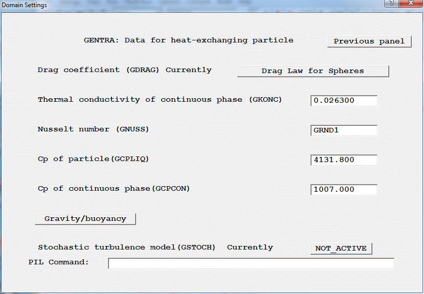
Figure 2.9: Data for heat-exchanging particles

The selection of drag coefficient is identical to that for the case of isothermal particles; see subsection (c) above for a complete explanation.
- Thermal conductivity of continuous phase. This option must be selected. A value of 0.0263 W/m/k is given as the default, corresponding to air at STP. If the user wishes to include his own temperature-dependent function for the thermal conductivity of the continuous phase, he should do the following:
1. Replace the constant value in the menu with a GRND number (i.e. GRND1).

2. Modify function routine GPROPS in the file GENTRA.FTN by adding coding in the relevant section. For this case, the coding should be added in the section commencing "GROUND1", and in the subsection commencing "3 Thermal Conductivity of the continuous phase". Coding relating the thermal conductivity (GPROPS) to the continuous-phase temperature (PARAMT) should then be inserted.

3. Before running EARTH, the GENTRA file will have to be recompiled and the EARTH executable relinked.
- The Nusselt number is defaulted to GRND1. This implies that the Nusselt number will be calculated from the correlation of equation (6.8); other correlations may be included in GPROPS following a procedure similar to that outlined above for the setting of the continuous-phase thermal conductivity. Alternatively, the Nusselt number may immediately be specified as a constant during this menu session.
- The specific heat capacity of the particle is defaulted to 4131.8 J/kg/k, which is representative of liquid water. Other constant values can be substituted for this or it can be replaced by a particle-temperature-dependent function in GPROPS.
- A constant value of 1007 J/kg/k is provided as the default value for the specific heat capacity of the continuous phase, this being the value for air at STP. The constant value can be altered during the menu session, or a temperature-dependent function can be implemented using the techniques mentioned above.
Gravity and buoyancy/pressure gradient effects and turbulent dispersion can be included; the reader is referred to the entries in sub-sections (c) and (a) above, for an explanation.
Data for melting/solidifying particles

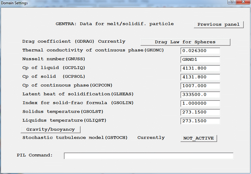
Figure 2.10: Data for melting/solidifying particles

The data required for melting/solidifying particles is as follows:
- Drag coefficient (see Subsection (c) for explanation).
- Thermal conductivity of continuous phase. The default value of 0.0263 is for air at STP.
- Nusselt number (see Subsection (d) for explanation).
- Cp of liquid phase of the melting/solidifying particle. The value of 4131.8 is representative of water.
- Cp of solid phase of the melting/solidifying particle.
- Cp of continuous phase.
- Latent heat of solidification. The default value of 3.335E+05 is for the formation of water ice. If the specific heat capacities of the liquid and solid phases were not identical, and if the change of phase was not isothermal, the latent heat of solidification would be temperature dependent, and a function would be required for it in GPROPS. Further explanation of this is provided in Section 6.3.4.
- Index for solid fraction formula (equation (6.15)). For the case of isothermal phase change, this variable is not employed.
- Solidus temperature of particle. The maximum temperature at which the particle is completely in the solid phase. The default value is for water.
- Liquidus temperature of particle. The minimum temperature at which the particle is completely in the liquid phase. The default value is for water.
- Gravity/buoyancy/pressure forces. (See Subsection (c) above for this option).
- Stochastic turbulence model. (See Subsection (a) above for details on this option).
The constant values which appear in this menu can be replaced with functions set in function routine GPROPS, according to the method described in Subsection (c) above.
Data for vaporising droplets

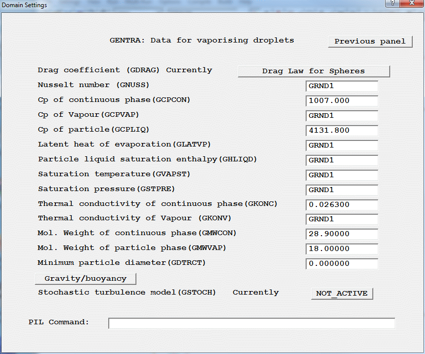
Figure 2.11: Data for vaporising droplets
- Drag coefficient. (See Subsection (c) for explanation.)
- Nusselt number. (See Subsection (d) for explanation.)
- Cp of Continuous phase. The default value of 1007 is for air at STP.
- Cp of Vapour. The value of CV is defaulted to GRND1, which directs control to GPROPS where a temperature-dependent property is specified.
- Cp of Particle. The default value of 4131.8 is for water.
- Latent heat of evaporation. A saturation-temperature-dependent function for the latent heat of evaporation is provided as the default value, GRND1. The function is for water vapour, and is derived from curve-fits on steam tables.
- Particle liquid saturation enthalpy. The default value of GRND1 produces a temperature-dependent function for the liquid saturation enthalpy of water, based on curve fits from steam tables.
- Saturation temperature of vapour. The default value of GRND1 provides a function for the saturation temperature of water vapour as a function of pressure.
- Saturation pressure of vapour. The default value of GRND1 provides the temperature-dependent vapour pressure correlation of Bain (1964).
- Thermal conductivity of continuous phase. The default value of 0.0263 is for air at STP.
- Thermal conductivity of vapour. The default value of GRND1 provides a temperature-dependent function for water vapour based on curve-fits to steam tables.
- Molecular weight of continuous-phase, defaulted to air (28.9).
- Molecular weight of particle phase, defaulted to water (18.0).
- Minimum particle diameter. The minimum size of particle below which the particle is assumed to have completely evaporated.
- Gravity/buoyancy/pressure forces. (See Subsection (c) above for details on this option.)
- Stochastic turbulence model. (See Subsection (a) above for details on this option.) This option appears on the next panel, reached by clicking Page down, or Line down.
The constant values, which appear in this menu, can be replaced with functions set in function routine GPROPS, according to the method described in Subsection (c) above.

Boundary conditions for particles

The Boundary conditions button in the Main Menu panel (figure 2.2) is used to specify the boundary conditions for the particles. Boundary conditions fall into the following categories:-

Inlets: The injection position and the particle properties (eg, velocities, diameter, temperature, etc) at the inlet must be given;
Exits: The boundary regions at which the particles can leave the domain must be specified;
Symmetry surfaces: The location of the symmetry surfaces (at which particles must be reflected) must be supplied;
Wall/obstacles: The behaviour of the particle following the collision with a wall or obstacle is selected from a range of choices (such as bouncing, sticking or flash vaporisation).

* Click on Boundary conditions to bring up the Boundary conditions panel.

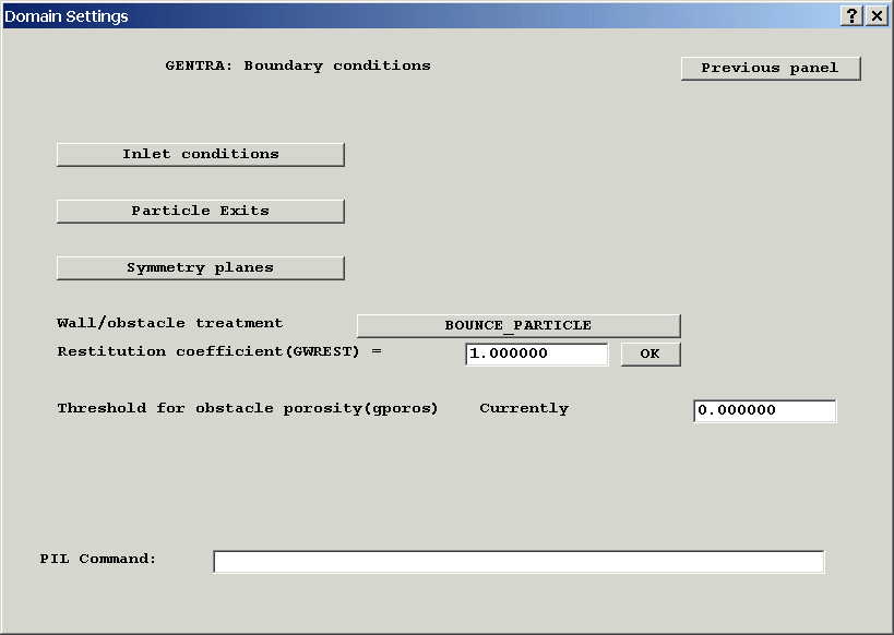
Figure 2.12: Boundary conditions for particles

The options in the Boundary conditions panel (shown in figure 2.12) are dealt with in subsequent subsections.

Inlet conditions

The Inlet conditions option of the Boundary conditions panel produces the panel in figure 2.13.

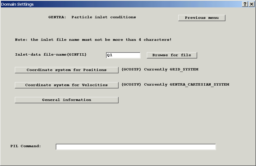
Figure 2.13 Particle inlet conditions

Inlet-data file-name. The inlet data in GENTRA is specified in a table located in an inlet-data file. The user can select the name of the inlet-data file through this option (the maximum length of the file name is 4 characters). Further information on the contents and format of the inlet data can be found at the end of this sub-section.

* The default file-name, Q1, will be used for the worked example.

Coordinate system for Positions. (Option not available in the present version of GENTRA.)

This option allows the specification of inlet co-ordinates in the inlet file in either the GENTRA Cartesian system (see glossary entry for a definition) or in the grid system. The distinction is only relevant to cylindrical-polar grids, since in Cartesian and BFC the GENTRA Cartesian system and the grid system coincide.

At present, the particle positions must be specified in the grid co-ordinate system. Thus for cylindrical-polar grids, the co-ordinates are specified as ?, r, z. The alignment between the Cartesian and polar grid systems is explained in Appendix H.

Coordinate system for Velocities (Option not available in the present version of GENTRA.)

This option allows the specification of inlet velocities in the inlet file in either the GENTRA Cartesian system (see glossary entry for a definition) or in the grid system. The distinction is only relevant to cylindrical-polar and BFC grids, since in Cartesian grids the velocity components in the GENTRA Cartesian system and in the grid system are the same.

At present, all inlet velocities must be specified in the Cartesian co-ordinate system, in the order Ucrt, Vcrt, Wcrt, where these represent the velocity components in the Cartesian X, y and Z directions respectively. For cylindrical-polar grids, the order of specification is Vcrt, Ucrt and Wcrt.

Format and contents of the inlet-data table

Inlet data In the inlet-data table, each parcel of particles has a data line; the data required is case-dependent. For the user's guidance, the GENTRA menu will generate, as a comment in the resulting Q1 file, a suitable heading for the inlet table.

The contents of the inlet table are also provided below for the different particle types.

Particle	Properties required
Lazy	POSTN
Stubborn	POSTN VELOC
Isothermal	POSTN VELOC DIAM DENSTY FRATE (NUMB)
Heat-exchanging	POSTN VELOC DIAM DENSTY FRATE TEMP (NUMB)
Melt/solidifying	POSTN VELOC DIAM LIQDEN FRATE TEMP SOLDEN (NUMB)
Vaporising	POSTN VELOC DIAM DENSTY FRATE TEMP (NUMB)

In the table above,

POSTN is the parcel inlet-position, in the co-ordinate system selected by the user (for one- or two-dimensional cases, no co-ordinates are needed for the dimensions for which the number of cells are one);
VELOC is the parcel inlet velocity-components, in the co-ordinate system selected by the user (for one- or two-dimensional cases, no components are needed for the dimensions in which the number of cells are one);
DIAM is the particle diameter;
DENSTY is the density of the particle; LIQDEN is the density of the liquid phase in solidifying particles (Units: kg/m3);
FRATE is the mass-flow rate of particles (Units: kg/s)
TEMP is the particle temperature (in K);
SOLDEN is, for melting/solidifying particles, the solid-phase density.
(NUMB) is an optional parameter, indicating the number of parcels of the given characteristics to be released from that position. When the stochastic turbulence model is active, GENTRA will track every parcel separately. When the stochastic turbulence model is inactive, GENTRA will simply multiply the mass-flow rate by the number of parcels and track a single parcel. When the NUMB data-item is missing, one parcel is assumed.
Comments Those lines in the inlet table containing, in any position, an asterisk (*) are treated as comments. The table heading can be inserted in this way in the data file. Blank lines are also ignored.
Line length The maximum length of an inlet-table line is 132 characters.
Number formatting The formatting of the numbers in the inlet table is free, but items of data must be separated with spaces ( ), commas (,) or semi-colons (;).
Error trapping GENTRA will skip those data lines that contain invalid characters (such as letter O instead of number zero), or that have a different number of data items to that which is required.

Q1 file as input file

By setting the inlet-data file-name to Q1 (the default), GENTRA will expect the inlet-data table to be in the Q1 file. All of the format rules for the inlet-data table (listed above) apply to the Q1 file. In addition, when the inlet data-table is in the Q1 file, the following practices must be observed:-

Inlet-data lines must be PIL comments; i.e., they must not start in the first or second column of the Q1 file, since they would be treated as commands by the SATELLITE.
The inlet-data table must be preceded and terminated by two special marks (also inserted as PIL comments). These marks are: <GENTRA-INLET-DATA> and <END-GENTRA-INLET> respectively.
WARNING: The maximum length of the inlet-data line is 132 characters. However, users are advised that the maximum length of a Q1-file line for the SATELLITE is 68 characters; if the SATELLITE is run after the inlet data has been inserted, and, following instructions from the user, the Q1 file is re-written, all the data items in columns 68 onwards will be lost.

The inlet-data table can be located anywhere in the Q1 file, and is normally written using a system file-editor after the menu session.

Note: GENTRA can generally cope with inlets lying exactly on the boundaries of the domain or on the grid pole; it is nevertheless a good practice to offset the inlet position by a small distance (e.g., 10-4 m).

* In this worked example, we will write the data table after finishing the menu session

Editing the File Containing the Input Data Table

In the VR-Environment, the file containing the inlet data table can be opened for editing by clicking on ‘File’, ‘Open file for editing’.

If the inlet data table is in Q1, select ‘Q1’, and then click ‘Yes’ to save the current settings to Q1. After editing the inlet data table, save the file and exit the editor. Click ‘Yes’ to reload the Q1 into VR-Editor, otherwise the new data will be lost.

To open any other file, select ‘Any file’, then open it from within the editor.

The editor used can be selected from ‘Options’, ‘Text file editor’.

Exits

Particle exits in GENTRA are represented through PATCH commands. Particle exit-PATCHes must have names beginning with GX, and be of an area type (ie, EAST, WEST, NORTH, SOUTH, HIGH, LOW).

In the VR Environment, all Inlet and Outlet objects act as GENTRA exits by default – the PATCHes they create all have names starting with GX. This behaviour can be altered by the ‘Acts as GENTRA exit’ buttons at the foot of the Inlet and Outlet object attribute dialogs. Note that these buttons only appear once GENTRA is active. The buttons can be seen in Figure 2.14.

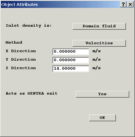
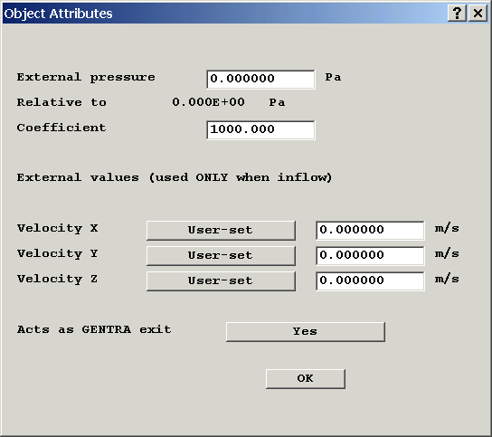
Figure 2.14: Inlet and Outlet attribute dialogs

To create an exit where only particles can leave the domain, set the coefficient for the pressure to zero in the Outlet attributes dialog. This will prevent the continuous phase from passing through.

Symmetry surfaces

The treatment for particles at an axis/surface of symmetry is always reflection (i.e., bouncing with a restitution coefficient of 1), regardless of the wall treatment selected for the problem.

GENTRA will automatically detect symmetry axes in the following two circumstances:

In 2D cylindrical-polar cases, and 3D cylindrical-polar cases in which the domain covers less than 2p radians in the circumferential direction, the grid pole is treated as an axis of symmetry.
In "wedge-like" 2D BFC domains (in which one of the domain sides collapses to a line), the edge of the wedge is treated as a symmetry axis.

In all other cases, axes/surfaces of symmetry must be declared by the user, so that GENTRA can act appropriately when a particle hits the axis/surface.

Symmetry surfaces in GENTRA are represented through PATCH commands whose PATCH name starts with GS. Each symmetry PATCH has also an associated PATCH type. This indicates on which face of the cells covered by the PATCH the symmetry surface is. The PATCH type can be EAST, WEST, NORTH, SOUTH, HIGH or LOW.

In the VR Environment, GENTRA symmetry surfaces are created by making a new object, with type GENTRA_SYMMETRY. This object type is only available when GENTRA is active. The PATCH created by such an object will have a name starting with GS, and will be of the correct type.

* The grid in the worked example is of the "wedge-like" kind; the axis will therefore be automatically detected by GENTRA.

Wall/obstacle treatment

The option Wall/obstacle treatment in the Boundary conditions panel (figure 2.12) specifies how the particle interacts with walls and obstacles (e.g., bouncing, sticking, removal).

See the GENTRA Glossary for a definition of wall/obstacle.

The options available depend on the type of particle; the user is therefore advised to set the particle type before visiting this menu. (The panel in figure 2.15 shows all of the possible treatments.)

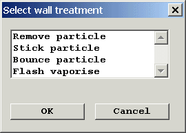
Figure 2.15: Wall/obstacle treatment

The menu Wall/obstacle treatment has, in the general case, the following options (figure 2.15):

Remove particle from domain. On hitting a wall or obstacle, the particle will be removed from the domain (ie, the tracking algorithm will abandon the particle and move on to the next one).
Stick particle to the wall. On hitting a wall or obstacle, the particle will remain stationary, but it will still undergo heat- and mass-transfer processes if the particle type allows for these.

(Note that REMOVE PARTICLE and STICK PARTICLE have the same effect for isothermal particles.)

Bounce particle off the wall. On hitting a wall or obstacle, the particle will be bounced. A restitution coefficient must be provided. The restitution coefficient is the absolute value of the ratio between the velocity component normal to the wall before and after the contact. The restitution coefficient must be greater than 0 and less than or equal to 1.

See Section 6.6.2 for more information on bouncing.

* Choose Bounce and set a restitution coefficient of 0.75 for the worked example. Then return to the previous panel.

Flash vaporisation. On hitting a wall or obstacle, the particle will be vaporised instantly, and all the mass will be transferred to the continuous phase.

This option is available only for VAPORISING DROPLETS.

Threshold for obstacle porosity

This option of the Boundary conditions panel (figure 2.12) allows the user to set the level of porosity that will be considered by GENTRA to constitute an obstacle for the particles.

For instance, a value of 0.75 will indicate that cells and cell faces with porosities between 0.0 and 0.75 will be taken as obstacles for the particulate phase.

Only values between 0 and 0.999 are accepted.

Numerical controls

The option Numerical controls of the main menu (figure 2.2) allows the user to control the solution procedure for the particulate phase. Users can, for instance:-
- Delay the first call to GENTRA until the continuous-phase flow-field has settled;
- Specify a frequency for calls to GENTRA;
- Set timeout limits for the particle flights;
- Apply relaxation to the interphase sources;
  
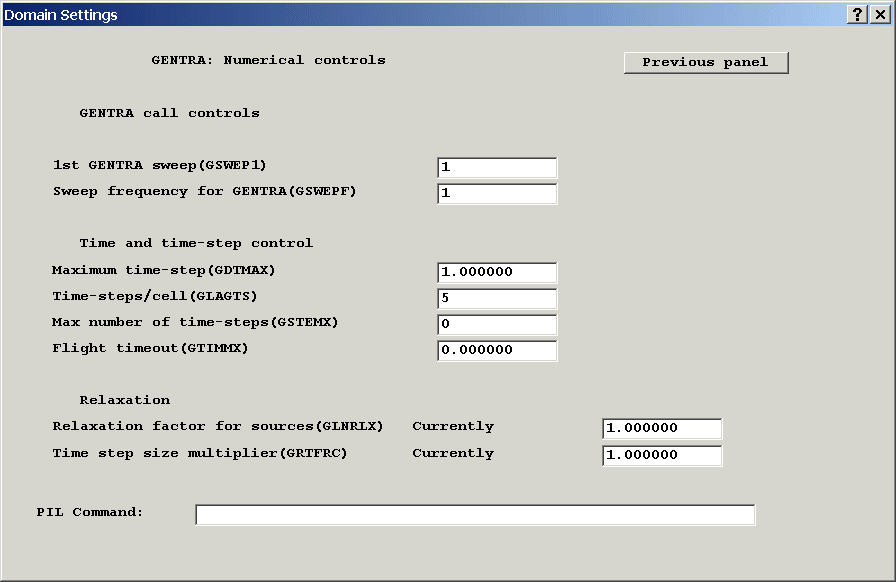
  Figure 2.16: Numerical controls
- 1st GENTRA sweep. This option allows the user to set the first EARTH sweep at which GENTRA will be called.
  It is often a good practice to start the particle tracking when the continuous-phase field is developed. The selection of values greater than 1 for this option will have that effect.
  
  This option can also be used to switch off the particle tracking by setting a value greater than the number of PHOENICS sweep (LSWEEP). If GENTRA is deactivated in this fashion, all the GENTRA settings will be retained in the Q1. It will be possible to turn GENTRA on again later. If GENTRA is turned off from the Models panel, all GENTRA settings are cleared. To turn GENTRA back on would involve re-setting all the non-default values.
- Sweep frequency for GENTRA. This option sets the frequency (in terms of EARTH sweeps) for calls to GENTRA. For instance, a value of 5 will cause the particle tracking to be effected for those sweeps whose index is a multiple of 5, and greater than or equal to the user-specified first-GENTRA-sweep (see option 1 in this menu).
  Values greater than 1 are recommended, in conjunction with source relaxation, for high particle loadings; for the continuous phase is then able to "absorb" the interphase sources before the next call to GENTRA.
- Maximum time-step This option allows the user to specify a maximum Lagrangian time-step, which will not be exceeded by GENTRA. (Note, however, that this time step may be reduced by GENTRA according to particle position and flow conditions.)
- Time-steps/cell. This option sets the approximate number of integration steps for each particle within each cell. A value of 5 is recommended. Note that this number can be increased (and occasionally reduced) by GENTRA according to flow conditions. (See Section 6.5.1)
- Max number of time-steps. This option allows the user to specify a maximum number of Lagrangian time-steps. If this limit is reached during the tracking of a particle, the particle is abandoned, a timeout message is issued and GENTRA moves on to the next particle.
  This device can, for instance, avoid large computing times arising from very small time-steps.
  
  The step number n can be positive, negative or zero:-
- Flight timeout. This option allows the user to specify a time limit for the tracking. If this limit is reached during the tracking of a particle, the particle is abandoned, a timeout message is issued and GENTRA moves on to the next particle.
  This device can avoid large computing times arising, for instance, from particles being trapped in recirculation regions.
  
  The timeout value r can be positive, negative or zero:-
- Relaxation factor for sources. This option allows the user to specify a linear-relaxation factor (a real number between 0 and 1) for the sources that account, in the continuous-phase equations, for the transfer of momentum, mass and thermal energy from the particles.
  Values between 0 and 1 have the effect of setting the source to be a weighted average of the sources calculated at the current and previous sweeps i.e.:
This may be beneficial for the convergence of the continuous-phase solution when the source is changing significantly from sweep to sweep;
- a value of 1 applies no relaxation to the source, (ie only the source calculated at the current sweep is employed); and
- a value of 0 sets the source equal to that employed at the previous sweep (ie the source does not change).
* Set a relaxation factor of 0.7
Input/Output controls

This is the last option of the Main Menu Panel (figure 2.2), which controls the input and output data flow of GENTRA. When I/O controls is selected in the Main Menu Panel, the following panel will appear.

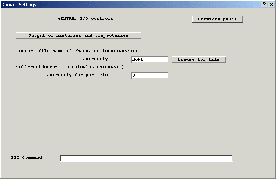
Figure 2.17: Input/Output controls
1. Output of history and trajectory
  - Selection of this option produces the panel of figure 2.18.
    
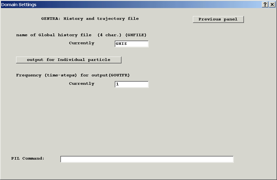
    Figure 2.18: History and trajectory files
    - name of the Global history file. Up to 4 characters can be given to the name of the file. Specifying "NONE" results in no global history file being written by the end of the GENTRA EARTH run.
    The global history file contains the results for all of the particles that are tracked. It can be post-processed using the UNPACK program to produce individual history and/or trajectory files. Details of the operation of the UNPACK program can be found in Appendix K.
    
    The Viewer can read the particle Global history file directly as a Macro, and will draw the tracks as streamlines. These can then be animated from the Streamline Management Dialog.
    - Output for Individual particle. The panel of figure 2.19 will follow if this option is selected.
    * We will require individual trajectory files so choose this option.
    
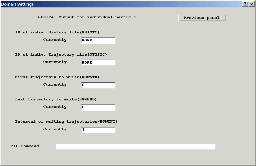
    Figure 2.19: Output for individual particle
    - ID of Indiv. history file: the first character for the name of the individual history file.
    - ID of Indiv. trajectory file: the first character for the name of the individual trajectory file.
    - First trajectory to write: the first track for which an individual history/trajectory file is required.
    - Last trajectory to write: the last track for which an individual history/trajectory file is required.
    - Interval of writing trajectories at which the individual history/trajectory file is written between the two tracks selected in the last two options.
    - In this worked example, we would like to produce trajectory files for all five particles being tracked. Therefore, input a suitable character with which the file names should commence, say T. We require trajectory files for each of the first five particles, so select the first and last particles as 1 and 5 respectively. Now select Previous panel twice to return to the I/O controls menu panel.
    Note that a maximum of 20 trajectory, and 20 history files can be created in this way. Trajectory and history information for all particles is held in the global history file (see figure 2.18 and Appendix K).
2. Restart file name
  The name of the GENTRA restart file. This option is not relevant to steady-state cases. In a transient case, it is the name to which GENTRA writes the particle information at the end of the last time step. Files are also written each time an intermediate dump file is written. These can then be used to continue the run.
  
  When a restart is activated from the Time step setting dialog and GENTRA is active, the name of the GENTRA restart file will also be set.
3. Cell-residence-time and particle-volume-fraction calculation
  This option in the Output control panel selects a particle for which the cell residence-time will be calculated by GENTRA. The particle is identified by the user through the particle number. In addition to the particle number, two special numbers can be used as flags to perform special functions:-
  
  0 will deactivate the calculation of residence time;
  
  -1 will add the residence time of all the particles in each cell.
  
  -2 will activate the calculation of a "particle volume-fraction" for each cell, representing the fraction of the cell volume occupied by particles. See Section 6.6.4 for additional details.
4. Particle-mass-concentration calculation
  This option in the Output control panel provides for the calculation of the particle mass concentration for each cell (see Section 6.6.5). It can also be activated by setting STORE(PMCO) in the Q1 input file.
5. Mixture-density calculation
  This option in the Output control panel provides for the calculation of the mixture density for each cell (see Section 6.6.6). It can also be activated by setting STORE(RHMX) in the Q1 input file.
6. Particle-mass-fraction calculation
  This option in the Output control panel provides for the calculation of the particle mass fraction for each cell (see Section 6.6.7). It can also be activated by setting STORE(PMFR) in the Q1 input file.
Ending the GENTRA Menu session

The GENTRA Menu session is ended from the GENTRA Main Menu Panel, shown in figure 2.2 by clicking on Previous panel. This returns control to the normal VR Main menu.

* Choose this option now to finish. Click on ‘Top’ and ‘OK’ to quit the VR Main Menu. Now edit the Q1 file and insert, as comments, the inlet data for the particles. The inlet data must be inserted between the marks <GENTRA-INLET-DATA> and <END-GENTRA-INLET> in the Q1 file. Refer to Section 2.7.1.3 above for instructions, and to the Q1 file in Appendix E for an example. Copy the settings from Appendix E.
The GENTRA Library

GENTRA has a library of ready-to-run examples and tests. To see the contents of the GENTRA Input Library, click on File, Load from Libraries on the VR Environment top menu.

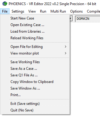
Figure 2.20: Accessing the Libraries

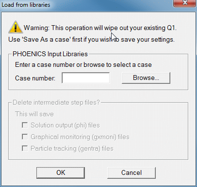
On the library dialog, click on Browse, then open the Option Libraries branch of the library tree. The GENTRA libraries are further subdivided as shown in Figure 2.21

Figure 2.21: The GENTRA Input Library

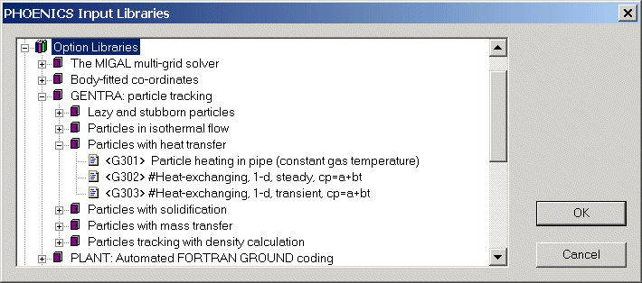
The contents of the Library are listed as Appendix F of this Guide.

Once the GENTRA Menu session is ended, or a library case has been loaded, you are ready to execute the calculating program EARTH. Chapter 4 explains how to do so. (You can skip Chapter 3, which gives additional details on data input using PIL, if you are a beginner.)

Top Previous Next