The classical fluid mechanics problem of flow around a circular cylinder is a popular test case for computational fluid dynamics. In the present paper the laminar vortex shedding behind a cylinder, found in the Reynolds number regime of 40 < Re < 190 , is studied. The Reynolds number is defined as Re = u d / ν , where u is the free stream velocity, d the diameter of the cylinder and ν the kinematic viscosity.
Below Re = 40 the flow is steady, i.e. no vortex street is formed, and above Re ≈ 190 the vortex street becomes unstable and irregular. The frequency, n, of the vortex shedding is traditionally expressed in non-dimensional form through the Strouhal number. In the Reynolds number range studied in this paper it is well know that the Strouhal number increases with the Reynolds number.
An outline of the computational configuration studied is given below in Figure 1, with dimensions given relative to the diameter of the cylinder.
The objective of this study is to verify that PHOENICS predicts the laminar vortex street behind a circular cylinder correctly. In particular we want to demonstrate that PARSOL offers a powerful and accurate approach to the problem studied.
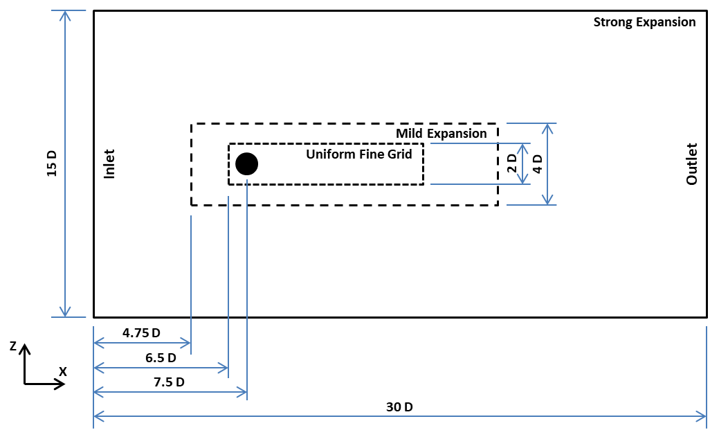 Figure 1
It will be assumed that the flow is transient, two-dimensional and laminar. We will further assume that the fluid is incompressible, with constant density, ρ, and kinematic viscosity, ν. The following set of equations is used:
Conservation of mass:
![]() (1)
(1)
Conservation of momentum:
 (2)
(2)
were p is pressure, ui denotes velocity and xi a coordinate.
Boundary conditions are given as a specified inflow a x = 0, see Figure 1, and a prescribed pressure at the outflow boundary. A no-slip boundary conditions is applied to the cylinder walls and at all other boundaries zero-friction is specified.
Quantities are normalised by the cylinder diameter, freestream velocity and reference density. With this normalisation the Reynolds number is specified with the viscosity alone.
The cylinder has a diameter of D = 1.0 and it's centre is located at (7.5 | 7.5). The computational domain (see Figure 1) has dimensions of 30 D by 15 D (x- and z-direction) with 227 cells in x and 98 in z, for a total of 22246 cells.
The "Uniform Fine Grid" region has the dimensions 9.5 x 2.0 D2 and a grid spacing of 1 / 16 D. This grid covers the cylinder and the expected wake-region. In the x-direction it starts 1 cylinder diameter upstream of the centre of the cylinder and in the y-direction the region's centre coincides the centre of the cylinder.
The "Mild Expansion" regions covers a slightly larger region, encompassing the "Uniform Fine Grid" region, with dimensions 14.5 x 4 D2. Expansion takes place along x and z away from the cylinder. This region starts 2.75 D upstream of the centre of the cyliner and is centered about the cylinder in z.
In the "Strong Expansion" region, away from the cylinder and its wake, the grid grows more rapidly in size along directions away from the cylinder.
The fluid is set to be a User-Defined fluid with a density of 1.0 and a kinematic viscosity of ν = 1 / Re. The inlet velocity is 1.0.
In order to reduce numerical diffusion the MINMOD scheme was used for the momentum equations.
Time step size was chosen such that the CFL number was 0.4 for the higher Reynolds number cases, and 0.64 for the lower Reynolds number cases. For Re = 10 and 30 the runs were stready.
Results will be presented for the Reynolds number interval 10 < Re < 150. In all simulations the cylinder diameter and inlet velocity were kept constant and the various Reynolds numbers were thus obtained by changing the viscosity.
In Figure 2 the vortex street at Re = 100 is illustrated. The colour filled contours were obtained from the solution of a scalar equation which had a value of 1.0 for the lower half of the inlet and 0.0 for the rest of the inlet.
A detailed view of the flow field behind the cylinder is given in Figure 3. For Re = 10 it is known that two small circulation regions form behind the cylinder (Tritton (1977)) and at Re = 30 these eddies have grown to a length of about two cylinder diameters. At Re = 40 the eddies become unstable and a vortex street is formed. The simulations show a periodic repetition at Re = 50 and hence predicts the instability at Re = 40, without any initialisation or perturbation. At Re = 100 the vortex street is well developed as can be seen in Figure 3.
The transverse velocity component was recorded, at the centreline, at the distance of about five diameters downstream the cylinder. In Figure 4 we see the result for two Reynolds numbers. As can be seen, a weak periodic flow is established also for Re = 50.
The transverse velocity recordings are used to determine the frequency, n, of the vortex shedding. With known cylinder diameter and free stream velocity we can then calculate the Strouhal number. In Thompson et al (1994) the experimentally determined relation between the Reynolds and Strouhal numbers is given as:
![]() (3)
(3)
where A = -3.3265, B = 0.1816 and C = 0.00016. This relation is believed to be accurate to ±1 % in the Reynolds number interval considered here. In Figure 5 this relation is shown together with present simulations. A fair agreement is found.
All results presented look plausible and are also in general agreement with experimental findings. In particular one can note the following features:
- The wake shape behind the cylinder for Reynolds numbers 10 and 30 (see Figure 3) is according to experimental evidence.
- The transition from a steady flow to the vortex shedding regime is predicted to take place between Re = 30 and Re = 50; also this is in agreement with experimental data.
- The variation of the Strouhal number with the Reynolds number is correctly predicted (see Figure 5).
The last point may need some further comments. In order for the points to be in good agreement with the curve at increasing Reynolds numbers the time step needs to be chosen smaller and the tolerance within a time step be more stringent. This may also be related to the transverse dimension of the domain, as it is known (Thompson et al (1994)) that the Strouhal number increases if the width decreases. We may thus have a too small width for the situation to be independent of the width. However, in this study no evaluation of the domain-size has been carried out. Further, solutions have been tested for time-step independence but not for grid independence. Some further work is thus required to establish that the solutions are domain-size and grid independent.
The general conclusion from the study is anyway that the laminar vortex shedding behind a circular cylinder is well predicted by PHOENICS.
POLIS. Documentation in the PHOENICS On-Line Information System.
Thompson M, Hourigan K, Sheridan J, 1994. Three-dimensional instabilities in the wake of a circular cylinder. Paper presented at the International Colloquium on Jets, Wakes and Shear Layer, DBCE, CSIRO, Highett, Victoria Australia.
Tritton D.J, 1977.Physical Fluid Dynamics. Van Nostrand Reinhold.
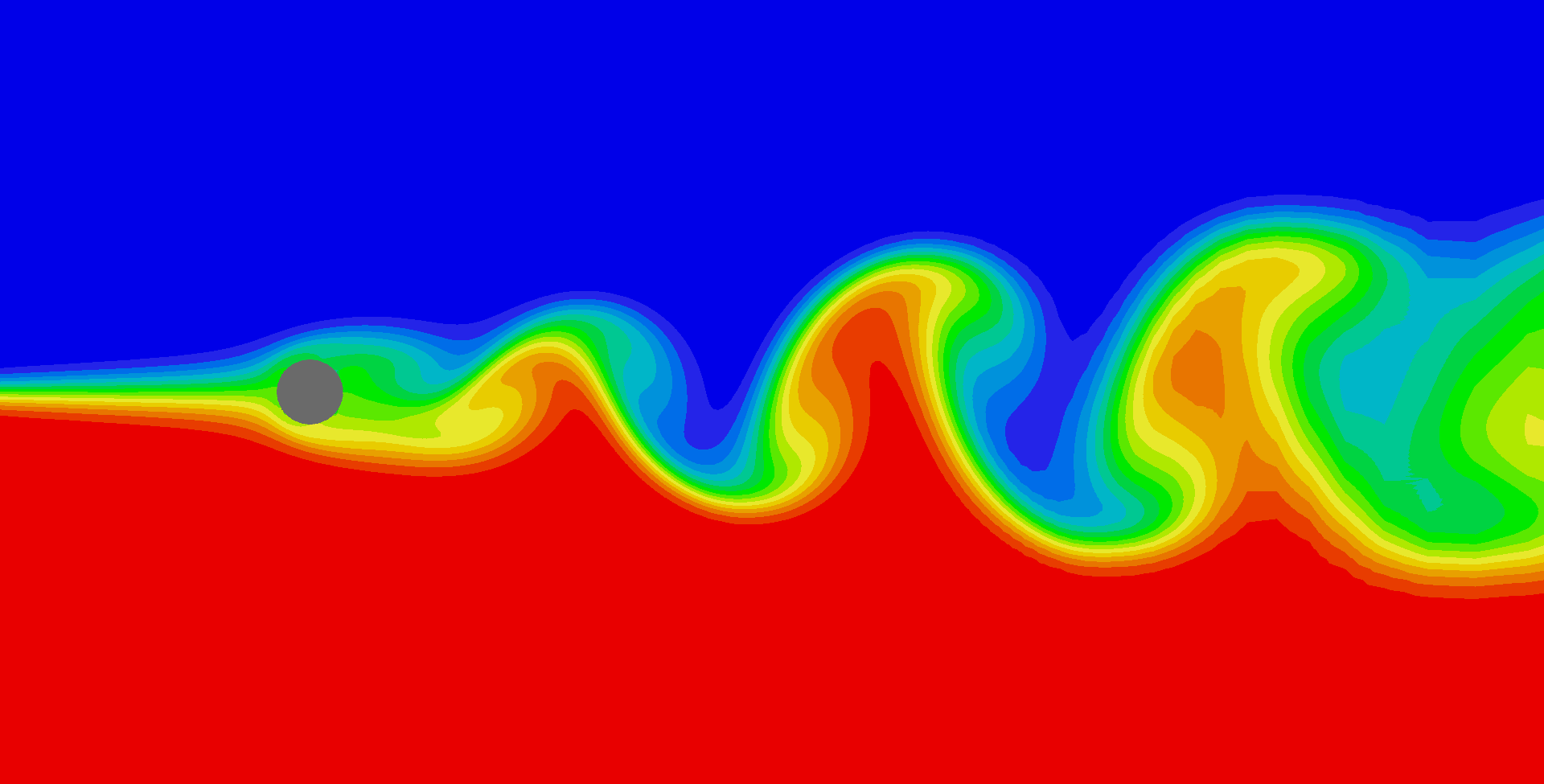 Figure 2. Flow field (top) and vortex
street for Re = 100.
Figure 2. Flow field (top) and vortex
street for Re = 100.
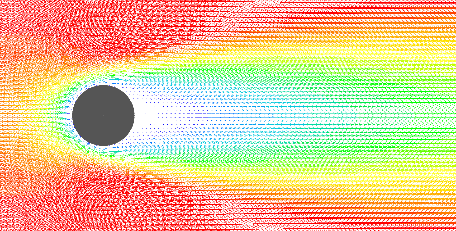 Figure 3a. Flow field behind the cylinder for Re = 10.
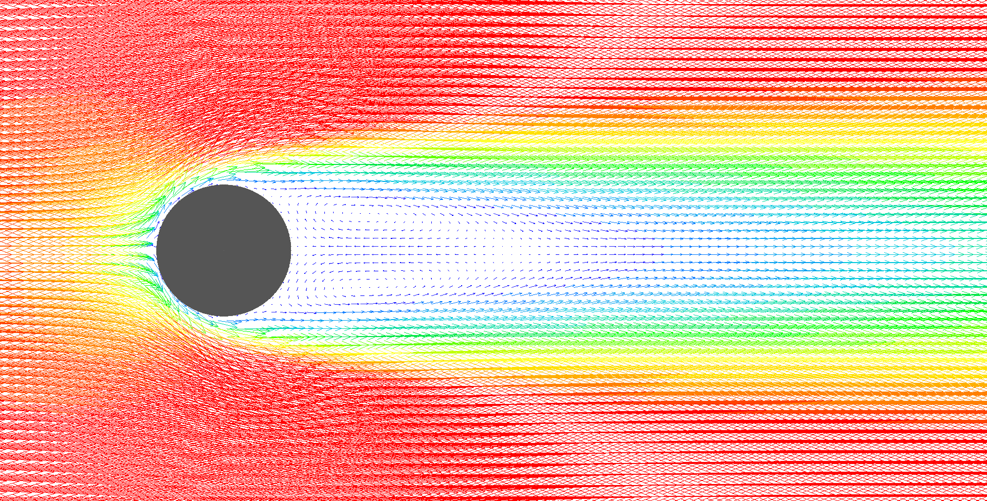 Figure 3b. Flow field behind the cylinder Re = 30.
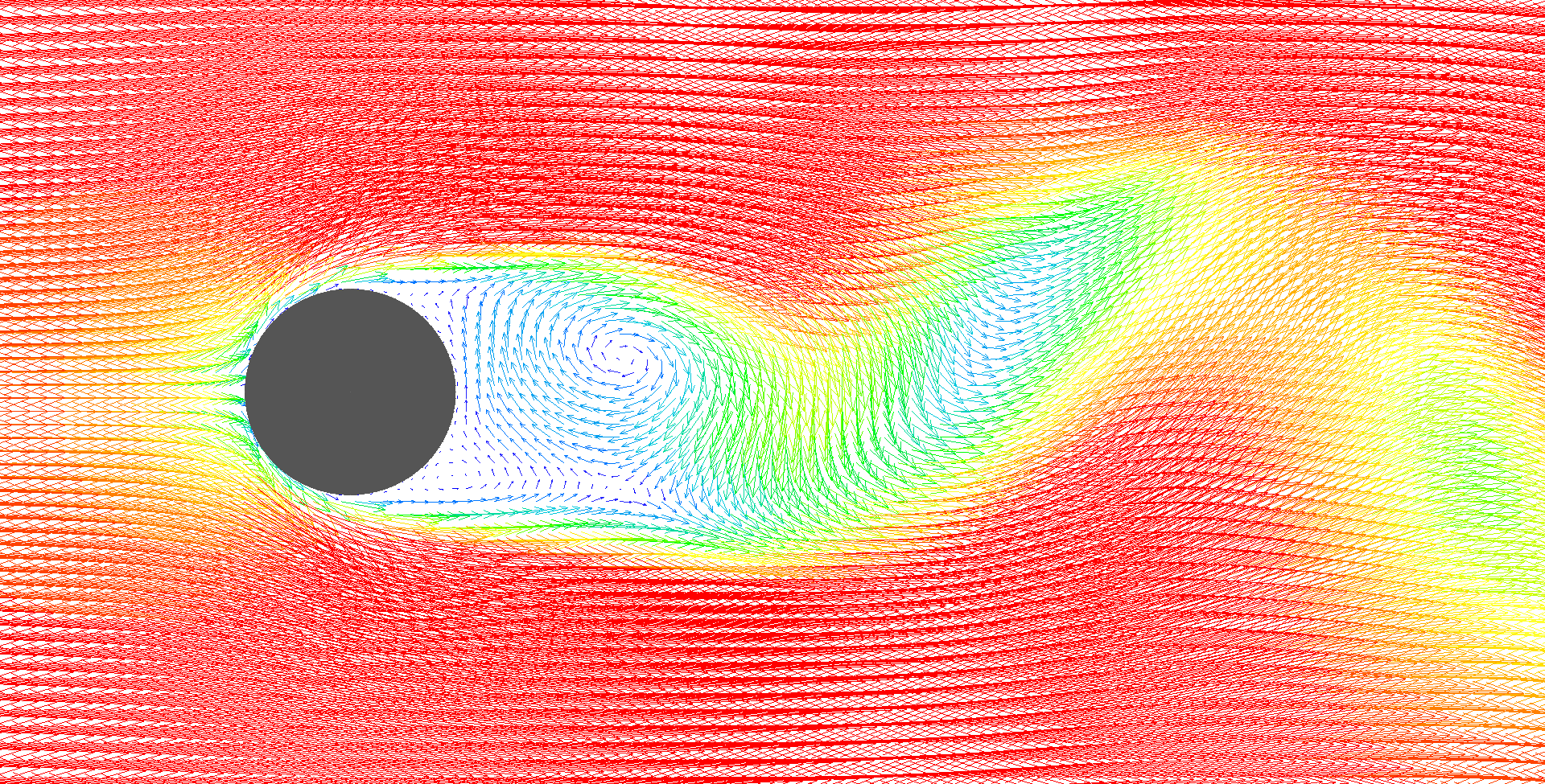 Figure 3c. Flow field behind the cylinder Re = 100.
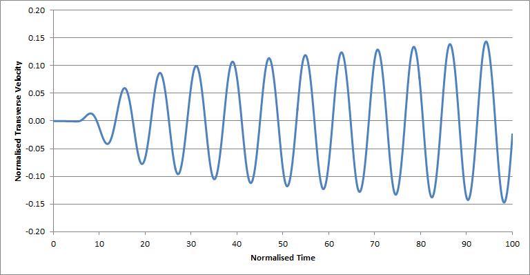 Figure 4a. Transverse velocity eight cylinder diameters behind the cylinder, at
Reynolds number = 50
Figure 4a. Transverse velocity eight cylinder diameters behind the cylinder, at
Reynolds number = 50
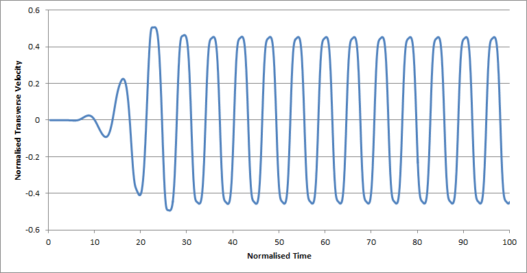 Figure 4b. Transverse velocity eight cylinder diameters behind the cylinder, at
Reynolds number = 100
Figure 4b. Transverse velocity eight cylinder diameters behind the cylinder, at
Reynolds number = 100
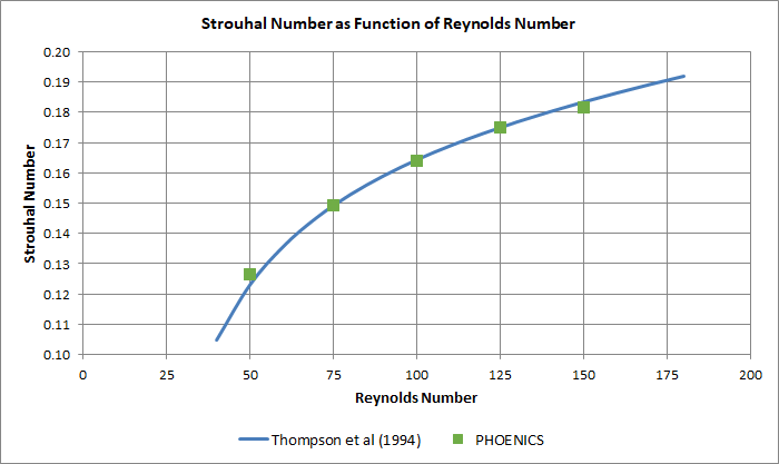 Figure 5. The Strouhal versus Reynolds number relation.
¾ experimental data, as given by Thompson et al (1994).
● present simulations.